Section 9 One-step correction
9.1 ☡ General analysis of plug-in estimators
Recall that \(\Algo_{Q_{W}}\) is an algorithm designed for the estimation of \(Q_{0,W}\) (see Section 7.3) and that we denote by \(Q_{n,W} \defq \Algo_{Q_{W}}(P_{n})\) the output of the algorithm trained on \(P_{n}\). Likewise, \(\Algo_{\Gbar}\) and \(\Algo_{\Qbar}\) are two generic algorithms designed for the estimation of \(\Gbar_{0}\) and of \(\Qbar_{0}\) (see Sections 7.4 and 7.6), \(\Gbar_{n} \defq \Algo_{\Gbar}(P_{n})\) and \(\Qbar_{n} \defq \Algo_{\Qbar}(P_{n})\) are their outputs once trained on \(P_{n}\).
Let us now introduce \(\Phat_n\) a law in \(\calM\) such that the \(Q_{W}\), \(\Gbar\) and \(\Qbar\) features of \(\Phat_n\) equal \(Q_{n,W}\), \(\Gbar_{n}\) and \(\Qbar_{n}\), respectively. We say that any such law is compatible with \(Q_{n,W}\), \(\Gbar_n\) and \(\Qbar_n\).
Now, let us substitute \(\Phat_n\) for \(P\) in (4.1):
\[\begin{equation} \tag{9.1} \Psi(\Phat_n) - \Psi(P_0) = - P_0 D^*(\Phat_n) + \Rem_{P_0}(\Phat_n) . \end{equation}\]
We show there in Appendix C.2 that, under conditions on the complexity/versatility of algorithms \(\Algo_{\Gbar}\) and \(\Algo_{\Qbar}\) (often referred to as regularity conditions) and assuming that their outputs \(\Gbar_{n}\) and \(\Qbar_{n}\) both consistently estimate their targets \(\Gbar_{0}\) and \(\Qbar_{0}\), it holds that
\[\begin{align} \Psi(\Phat_n) - \Psi(P_0) &= - P_{n} D^*(\Phat_n) + P_{n} D^*(P_0) + o_{P_0}(1/\sqrt{n}) \tag{9.2} \\ \notag &= - P_{n} D^*(\Phat_n)+ \frac{1}{n} \sum_{i=1}^n D^*(P_0)(O_i) + o_{P_0}(1/\sqrt{n}). \end{align}\]
In light of (3.7), \(\Psi(\Phat_{n})\) would be asymptotically linear with influence curve \(\IC=D^{*}(P_{0})\) in the absence of the random term \(-P_{n} D^*(\Phat_n)\). Unfortunately, it turns out that this term can degrade dramatically the behavior of the plug-in estimator \(\Psi(\Phat_{n})\).
9.2 One-step correction
Luckily, a very simple workaround allows to circumvent the problem. Proposed in (Le Cam 1969) (see also (Pfanzagl 1982) and (Vaart 1998)), the workaround merely consists in adding the random term to the initial estimator, that is, in estimating \(\Psi(P_0)\) not with \(\Psi(\Phat_n)\) but instead with \[\begin{equation} \psinos \defq \Psi(\Phat_n) + P_{n} D^*(\Phat_n) = \Psi(\Phat_n) + \frac{1}{n} \sum_{i=1}^{n} D^*(\Phat_n)(O_{i}). \tag{9.3} \end{equation}\]
Obviously, in light of (9.2), \(\psinos\) is asymptotically linear with influence curve \(\IC=D^{*}(P_{0})\). Thus, by the central limit theorem, \(\sqrt{n} (\psinos - \Psi(P_0))\) converges in law to a centered Gaussian distribution with variance \[\begin{equation} \Var_{P_0}(D^{*}(P_{0})(O)) = \Exp_{P_0}(D^{*}(P_{0})(O)). \end{equation}\]
The detailed general analysis of plug-in estimators developed there in Appendix C.2 also revealed that the above asymptotic variance is consistently estimated with \[\begin{equation} P_{n} D^{*}(\Phat_{n})^{2} = \frac{1}{n} \sum_{i=1}^{n} D^*(\Phat_n)^{2}(O_{i}). \end{equation}\] Therefore, by the central limit theorem and Slutsky’s lemma (see the argument there in Appendix B.3.1), \[\begin{equation*} \left[\psinos \pm \Phi^{-1}(1-\alpha) \frac{P_{n} D^{*}(\Phat_{n})^{2}}{\sqrt{n}}\right] \end{equation*}\] is a confidence interval for \(\Psi(P_0)\) with asymptotic level \((1-2\alpha)\).
9.3 Empirical investigation
In light of (9.3) if the estimator equals \(\Psi(\Phat_{n})\),
then performing a one-step correction essentially boils down to computing two
quantities, \(-P_{n} D^{*}(\Phat_{n})\) (the bias term) and \(P_{n} D^{*}(\Phat_{n})^{2}\) (an estimator of the asymptotic variance of
\(\psinos\)). The tlrider package makes the operation very easy thanks to the
function apply_one_step_correction.
Let us illustrate its use by updating the G-computation estimator built on the
\(n=1000\) first observations in obs by relying on \(\Algo_{\Qbar,\text{kNN}}\),
that is, on the algorithm for the estimation of \(\Qbar_{0}\) as it is
implemented in estimate_Qbar with its argument algorithm set to the
built-in kknn_algo (see Section 7.6.2). The algorithm has
been trained earlier on this data set and produced the object Qbar_hat_kknn.
The following chunk of code re-computes the corresponding G-computation
estimator, using again the estimator QW_hat of the marginal law of \(W\) under
\(P_{0}\) (see Section 7.3), then applied the one-step correction:
(psin_kknn <- compute_gcomp(QW_hat, wrapper(Qbar_hat_kknn, FALSE), 1e3))
#> # A tibble: 1 × 2
#>   psi_n   sig_n
#>   <dbl>   <dbl>
#> 1 0.101 0.00306
(psin_kknn_os <- apply_one_step_correction(head(obs, 1e3),
                                           wrapper(Gbar_hat, FALSE),
                                           wrapper(Qbar_hat_kknn, FALSE),
                                           psin_kknn$psi_n))
#> # A tibble: 1 × 3
#>    psi_n  sig_n    crit_n
#>    <dbl>  <dbl>     <dbl>
#> 1 0.0999 0.0171 -0.000633
In the call to apply_one_step_correction we provide (i) the data set at
hand (first line), (ii) the estimator Gbar_hat of \(\Gbar_{0}\) that we
built earlier by using algorithm \(\Algo_{\Gbar,1}\) (second line; see Section
7.4.2), (iii) the estimator Qbar_hat_kknn of \(\Qbar_{0}\)
and the G-computation estimator psin_kknn that resulted from it (third and
fourth lines).
To assess what is the impact of the one-step correction, let us apply the
one-step correction to the estimators that we built in Section
8.4.3. The object learned_features_fixed_sample_size
already contains the estimated features of \(P_{0}\) that are needed to perform
the one-step correction to the estimators \(\psi_{n}^{d}\) and \(\psi_{n}^{e}\),
namely, thus we merely have to call the function apply_one_step_correction.
psi_hat_de_one_step <- learned_features_fixed_sample_size %>%
  mutate(os_est_d =
           pmap(list(obs, Gbar_hat, Qbar_hat_d, est_d),
                ~ apply_one_step_correction(as.matrix(..1),
                                 wrapper(..2, FALSE),
                                 wrapper(..3, FALSE),
                                 ..4$psi_n)),
         os_est_e =
           pmap(list(obs, Gbar_hat, Qbar_hat_e, est_e),
                ~ apply_one_step_correction(as.matrix(..1),
                                 wrapper(..2, FALSE),
                                 wrapper(..3, FALSE),
                                 ..4$psi_n))) %>%
  select(os_est_d, os_est_e) %>%
  pivot_longer(c(`os_est_d`, `os_est_e`),
               names_to = "type", values_to = "estimates") %>%
  extract(type, "type", "_([de])$") %>%
  mutate(type = paste0(type, "_one_step")) %>%
  unnest(estimates) %>%
  group_by(type) %>%
  mutate(sig_alt = sd(psi_n)) %>%
  mutate(clt_ = (psi_n - psi_zero) / sig_n,
         clt_alt = (psi_n - psi_zero) / sig_alt) %>%
  pivot_longer(c(`clt_`, `clt_alt`),
               names_to = "key", values_to = "clt") %>%
  extract(key, "key", "_(.*)$") %>%
  mutate(key = ifelse(key == "", TRUE, FALSE)) %>%
  rename("auto_renormalization" = key)

(bias_de_one_step <- psi_hat_de_one_step %>%
   group_by(type, auto_renormalization) %>%
   summarize(bias = mean(clt)) %>% ungroup)
#> # A tibble: 4 × 3
#>   type       auto_renormalization     bias
#>   <chr>      <lgl>                   <dbl>
#> 1 d_one_step FALSE                -0.0142
#> 2 d_one_step TRUE                 -0.0307
#> 3 e_one_step FALSE                 0.0126
#> 4 e_one_step TRUE                 -0.00460

fig <- ggplot() +
  geom_line(aes(x = x, y = y),
            data = tibble(x = seq(-4, 4, length.out = 1e3),
                          y = dnorm(x)),
            linetype = 1, alpha = 0.5) +
  geom_density(aes(clt, fill = type, colour = type),
               psi_hat_de_one_step, alpha = 0.1) +
  geom_vline(aes(xintercept = bias, colour = type),
             bias_de_one_step, size = 1.5, alpha = 0.5) +
  facet_wrap(~ auto_renormalization,
             labeller =
               as_labeller(c(`TRUE` = "auto-renormalization: TRUE",
                             `FALSE` = "auto-renormalization: FALSE")),
             scales = "free")

fig +
  labs(y = "",
       x = bquote(paste(sqrt(n/v[n]^{list(d, e, os)})*
                        (psi[n]^{list(d, e, os)} - psi[0]))))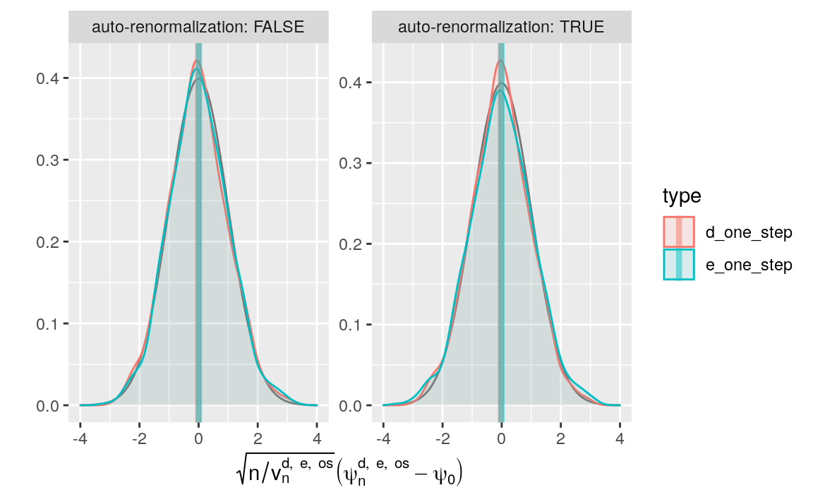
Figure 9.1: Kernel density estimators of the law of two one-step-G-computation estimators of \(\psi_{0}\) (recentered with respect to \(\psi_{0}\), and renormalized). The estimators respectively hinge on algorithms \(\Algo_{\Qbar,1}\) (d) and \(\Algo_{\Qbar,\text{kNN}}\) (e) to estimate \(\Qbar_{0}\), and on one-step correction. Two renormalization schemes are considered, either based on an estimator of the asymptotic variance (left) or on the empirical variance computed across the 1000 independent replications of the estimators (right). We emphasize that the \(x\)-axis ranges differ between the left and right plots.
It seems that the one-step correction performs quite well (in particular,
compare bias_de with bias_de_one_step):
bind_rows(bias_de, bias_de_one_step) %>%
  filter(!auto_renormalization) %>%
  arrange(type)
#> # A tibble: 4 × 3
#>   type       auto_renormalization    bias
#>   <chr>      <lgl>                  <dbl>
#> 1 d          FALSE                 0.234
#> 2 d_one_step FALSE                -0.0142
#> 3 e          FALSE                 0.107
#> 4 e_one_step FALSE                 0.0126
What about the estimation of the asymptotic variance, and of the mean squared-error of the estimators?
psi_hat_de %>%
  full_join(psi_hat_de_one_step) %>%
  filter(auto_renormalization) %>%
  group_by(type) %>%
  summarize(sd = mean(sig_n),
            se = sd(psi_n),
            mse = mean((psi_n - psi_zero)^2) * n()) %>%
  arrange(type)
#> # A tibble: 4 × 4
#>   type            sd     se   mse
#>   <chr>        <dbl>  <dbl> <dbl>
#> 1 d          0.00206 0.0171 0.309
#> 2 d_one_step 0.0173  0.0171 0.291
#> 3 e          0.00288 0.0172 0.298
#> 4 e_one_step 0.0166  0.0175 0.305
The sd (estimator of the asymptotic standard deviation) and se
(empirical standard deviation) entries are similar. This indicates that the
inference of the asymptotic variance of the one-step estimators based on the
influence curve is rather accurate for both the d- and e-variants that we
implemented. As for the mean square error, it is made respectively slightly
smaller or bigger or by the one-step update for type d and e, the
d_one_step estimator exhibiting the smallest mean square error.
9.4 ⚙ Investigating further the one-step correction methodology
Use
estimate_Gbarto create an oracle algorithm \(\Algora_{\Gbar,s}\) for the estimation of \(\Gbar_{0}\) that, for any \(s > 0\), estimates \(\Gbar_{0}(w)\) with \[\begin{equation*} \Gbar_{n}(w) \defq \Algora_{\Gbar,s} (P_{n})(w) \defq \expit\left(\logit\left(\Gbar_{0}(w)\right) + s Z\right) \end{equation*}\] where \(Z\) is a standard normal random variable.20 What would happen if one chose \(s=0\) in the above definition? What happens when \(s\) converges to 0? Explain why the algorithm is said to be an oracle algorithm.Use
estimate_Qbarto create an oracle algorithm \(\Algora_{\Qbar,s}\) for the estimation of \(\Qbar_{0}\) that, for any \(s > 0\), estimates \(\Qbar_{0}(a,w)\) with \[\begin{equation*} \Qbar_{n}(a,w) \defq \Algora_{\Gbar,s} (P_{n})(a,w) \defq \expit\left(\logit\left(\Qbar_{0}(a,w)\right) + s Z\right) \end{equation*}\] where \(Z\) is a standard normal random variable. The comments made about \(\Algora_{\Gbar,s}\) in the above problem also apply to \(\Algora_{\Qbar,s}\).Reproduce the simulation study developed in Sections 8.4.3 and 9.3 with the oracle algorithms \(\Algora_{\Gbar,s}\) and \(\Algora_{\Qbar,s'}\) substituted for used in these sections. Change the values of \(s,s' > 0\) and compare how well the estimating procedure performs depending on the product \(ss'\). What do you observe? We invite you to refer to Section C.2.1.
Note that the algorithm does not really to be trained.↩︎