$\newcommand{\bbO}{\mathbb{O}}$ $\newcommand{\bbD}{\mathbb{D}}$ $\newcommand{\bbP}{\mathbb{P}}$ $\newcommand{\bbR}{\mathbb{R}}$ $\newcommand{\Algo}{\widehat{\mathcal{A}}}$ $\newcommand{\Algora}{\widetilde{\mathcal{A}}}$ $\newcommand{\calF}{\mathcal{F}}$ $\newcommand{\calM}{\mathcal{M}}$ $\newcommand{\calP}{\mathcal{P}}$ $\newcommand{\calO}{\mathcal{O}}$ $\newcommand{\calQ}{\mathcal{Q}}$ $\newcommand{\defq}{\doteq}$ $\newcommand{\Exp}{\textrm{E}}$ $\newcommand{\IC}{\textrm{IC}}$ $\newcommand{\Gbar}{\bar{G}}$ $\newcommand{\one}{\textbf{1}}$ $\newcommand{\psinos}{\psi_{n}^{\textrm{os}}}$ $\renewcommand{\Pr}{\textrm{Pr}}$ $\newcommand{\Phat}{P^{\circ}}$ $\newcommand{\Psihat}{\widehat{\Psi}}$ $\newcommand{\Qbar}{\bar{Q}}$ $\newcommand{\tcg}[1]{\textcolor{olive}{#1}}$ $\DeclareMathOperator{\Dirac}{Dirac}$ $\DeclareMathOperator{\expit}{expit}$ $\DeclareMathOperator{\logit}{logit}$ $\DeclareMathOperator{\Rem}{Rem}$ $\DeclareMathOperator{\Var}{Var}$

Section 8 Two “naive” inference strategies

8.1 Why “naive?”

In this section, we present and discuss two strategies for the inference of $\Psi(P_{0})$. In light of Section 7.1, both unfold in two stages. During the first stage, some features among $Q_{0,W}$, $\Gbar_{0}$ and $\Qbar_{0}$ (the $\Psi$-specific nuisance parameters, see Section 7) are estimated. During the second stage, these estimators are used to build estimators of $\Psi(P_{0})$.

Although the strategies sound well conceived, a theoretical analysis reveals that they lack a third stage trying to correct an inherent flaw. They are thus said naive. The analysis and a first modus operandi are presented in Section 9.1.

8.2 IPTW estimator

8.2.1 Construction and computation

In Section 6.3, we developed an IPTW estimator, $\psi_{n}^{b}$, assuming that we knew $\Gbar_{0}$ beforehand. What if we did not? Obviously, we could estimate it and substitute the estimator of $\ell\Gbar_{0}$ for $\ell\Gbar_{0}$ in (6.3).

Let $\Algo_{\Gbar}$ be an algorithm designed for the estimation of $\Gbar_{0}$ (see Section 7.4). We denote by $\Gbar_{n} \defq \Algo_{\Gbar}(P_{n})$ the output of the algorithm trained on $P_{n}$, and by $\ell\Gbar_{n}$ the resulting (empirical) function given by

\[\begin{equation*} \ell\Gbar_{n}(A,W) \defq A \Gbar_{n}(W) + (1-A) (1 - \Gbar_{n}(W)). \end{equation*}\]

In light of (6.3), we introduce

\[\begin{equation*} \psi_{n}^{c} \defq \frac{1}{n} \sum_{i=1}^{n} \left(\frac{2A_{i} - 1}{\ell\Gbar_{n}(A_{i}, W_{i})} Y_{i}\right). \end{equation*}\]

From a computational point of view, the tlrider package makes it easy to build $\psi_{n}^{c}$. Recall that

compute_iptw(head(obs, 1e3), Gbar)

implements the computation of $\psi_{n}^{b}$ based on the $n=1000$ first observations stored in obs, using the true feature $\Gbar_{0}$ stored in Gbar, see Section 6.3.3 and the construction of psi_hat_ab. Similarly,

Gbar_hat <- estimate_Gbar(head(obs, 1e3), working_model_G_one)
compute_iptw(head(obs, 1e3), wrapper(Gbar_hat)) %>% pull(psi_n)
#> [1] 0.104

implements (i) the estimation of $\Gbar_{0}$ with $\Gbar_{n}$/Gbar_hat using algorithm $\Algo_{\Gbar,1}$ (first line) then (ii) the computation of $\psi_{n}^{c}$ (second line), both based on the same observations as above.

Note how we use function wrapper (simply run ?wrapper to see its man page).

8.2.2 Elementary statistical properties

Because $\Gbar_{n}$ minimizes the empirical risk over a finite-dimensional, identifiable, and well-specified working model, $\sqrt{n} (\psi_{n}^{c} - \psi_{0})$ converges in law to a centered Gaussian law. Moreover, the asymptotic variance of $\sqrt{n} (\psi_{n}^{c} - \psi_{0})$ is conservatively¹⁵ estimated with

\[\begin{align*} v_{n}^{c} &\defq \Var_{P_{n}} \left(\frac{2A-1}{\ell\Gbar_{n}(A,W)}Y\right) \\ &= \frac{1}{n} \sum_{i=1}^{n}\left(\frac{2A_{i}-1}{\ell\Gbar_{n} (A_{i},W_{i})} Y_{i} - \psi_{n}^{c}\right)^{2}. \end{align*}\]

We investigate empirically the statistical behavior of $\psi_{n}^{c}$ in Section 8.2.3. For an analysis of the reason why $v_{n}^{c}$ is a conservative estimator of the asymptotic variance of $\sqrt{n} (\psi_{n}^{c} - \psi_{0})$, see there in Appendix C.1.1.

Before proceeding, let us touch upon what would have happened if we had used a less amenable algorithm $\Algo_{\Gbar}$. For instance, $\Algo_{\Gbar}$ could still be well-specified¹⁶ but so versatile/complex (as opposed to being based on well-behaved, finite-dimensional parametric model) that the estimator $\Gbar_{n}$, though still consistent, would converge slowly to its target. Then, root-$n$ consistency would fail to hold. Or $\Algo_{\Gbar}$ could be mis-specified and there would be no guarantee at all that the resulting estimator $\psi_{n}^{c}$ be even consistent.

8.2.3 Empirical investigation

Let us compute $\psi_{n}^{c}$ on the same iter = 1000 independent samples of independent observations drawn from $P_{0}$ as in Section 6.3. As explained in Sections 5 and 6.3.3, we first make 1000 data sets out of the obs data set (third line), then train algorithm $\Algo_{\Gbar,1}$ on each of them (fifth to seventh lines). After the first series of commands the object learned_features_fixed_sample_size, a tibble, contains 1000 rows and three columns.

We created learned_features_fixed_sample_size to store the estimators of $\Gbar_{0}$ for future use. We will at a later stage enrich the object, for instance by adding to it estimators of $\Qbar_{0}$ obtained by training different algorithms on each smaller data set.

In the second series of commands, the object psi_hat_abc is obtained by adding to psi_hat_ab (see Section 6.3.3) an 1000 by four tibble containing notably the values of $\psi_{n}^{c}$ and $\sqrt{v_{n}^{c}}/\sqrt{n}$ computed by calling compute_iptw. The object also contains the values of the recentered (with respect to $\psi_{0}$) and renormalized $\sqrt{n}/\sqrt{v_{n}^{c}} (\psi_{n}^{c} - \psi_{0})$. Finally, bias_abc reports amounts of bias (at the renormalized scale).

learned_features_fixed_sample_size <-
  obs %>% as_tibble %>%
  mutate(id = (seq_len(n()) - 1) %% iter) %>%
  nest(obs = c(W, A, Y)) %>%
  mutate(Gbar_hat =
           map(obs,
               ~ estimate_Gbar(., algorithm = working_model_G_one)))

psi_hat_abc <-
  learned_features_fixed_sample_size %>%
  mutate(est_c =
           map2(obs, Gbar_hat,
                ~ compute_iptw(as.matrix(.x), wrapper(.y, FALSE)))) %>%
  unnest(est_c) %>% select(-Gbar_hat, -obs) %>%
  mutate(clt = (psi_n - psi_zero) / sig_n,
         type = "c") %>%
  full_join(psi_hat_ab)

(bias_abc <- psi_hat_abc %>%
   group_by(type) %>% summarize(bias = mean(clt), .groups = "drop"))
#> # A tibble: 3 × 2
#>   type      bias
#>   <chr>    <dbl>
#> 1 a      1.39   
#> 2 b      0.0241 
#> 3 c     -0.00454

By the above chunk of code, the average of $\sqrt{n/v_{n}^{c}} (\psi_{n}^{c} - \psi_{0})$ computed across the realizations is equal to -0.005 (see bias_abc). In words, the bias of $\psi_{n}^{c}$ is even smaller than that of $\psi_{n}^{b}$ despite the fact that the construction of $\psi_{n}^{c}$ hinges on the estimation of $\Gbar_{0}$ (based on the well-specified algorithm $\Algo_{\Gbar,1}$).

We represent the empirical laws of the recentered (with respect to $\psi_{0}$) and renormalized $\psi_{n}^{a}$, $\psi_{n}^{b}$ and $\psi_{n}^{c}$ in Figures 8.1 (kernel density estimators) and 8.2 (quantile-quantile plots).

fig_bias_ab +
  geom_density(aes(clt, fill = type, colour = type), psi_hat_abc, alpha = 0.1) +
  geom_vline(aes(xintercept = bias, colour = type),
             bias_abc, size = 1.5, alpha = 0.5) +
  xlim(-3, 4) + 
  labs(y = "",
       x = bquote(paste(sqrt(n/v[n]^{list(a, b, c)})*
                        (psi[n]^{list(a, b, c)} - psi[0]))))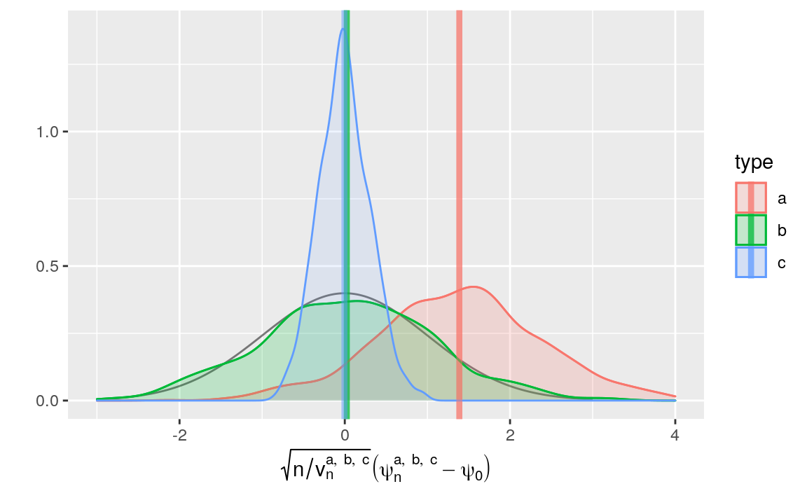

$Kernel density estimators of the law of three estimators of $\psi_{0}$ (recentered with respect to $\psi_{0}$, and renormalized), one of them misconceived (a), one assuming that $\Gbar_{0}$ is known (b) and one that hinges on the estimation of $\Gbar_{0}$ (c). The present figure includes Figure 6.1 (but the colors differ). Built based on 1000 independent realizations of each estimator.$

Figure 8.1: Kernel density estimators of the law of three estimators of $\psi_{0}$ (recentered with respect to $\psi_{0}$, and renormalized), one of them misconceived (a), one assuming that $\Gbar_{0}$ is known (b) and one that hinges on the estimation of $\Gbar_{0}$ (c). The present figure includes Figure 6.1 (but the colors differ). Built based on 1000 independent realizations of each estimator.

ggplot(psi_hat_abc, aes(sample = clt, fill = type, colour = type)) +
  geom_abline(intercept = 0, slope = 1, alpha = 0.5) +
  geom_qq(alpha = 1)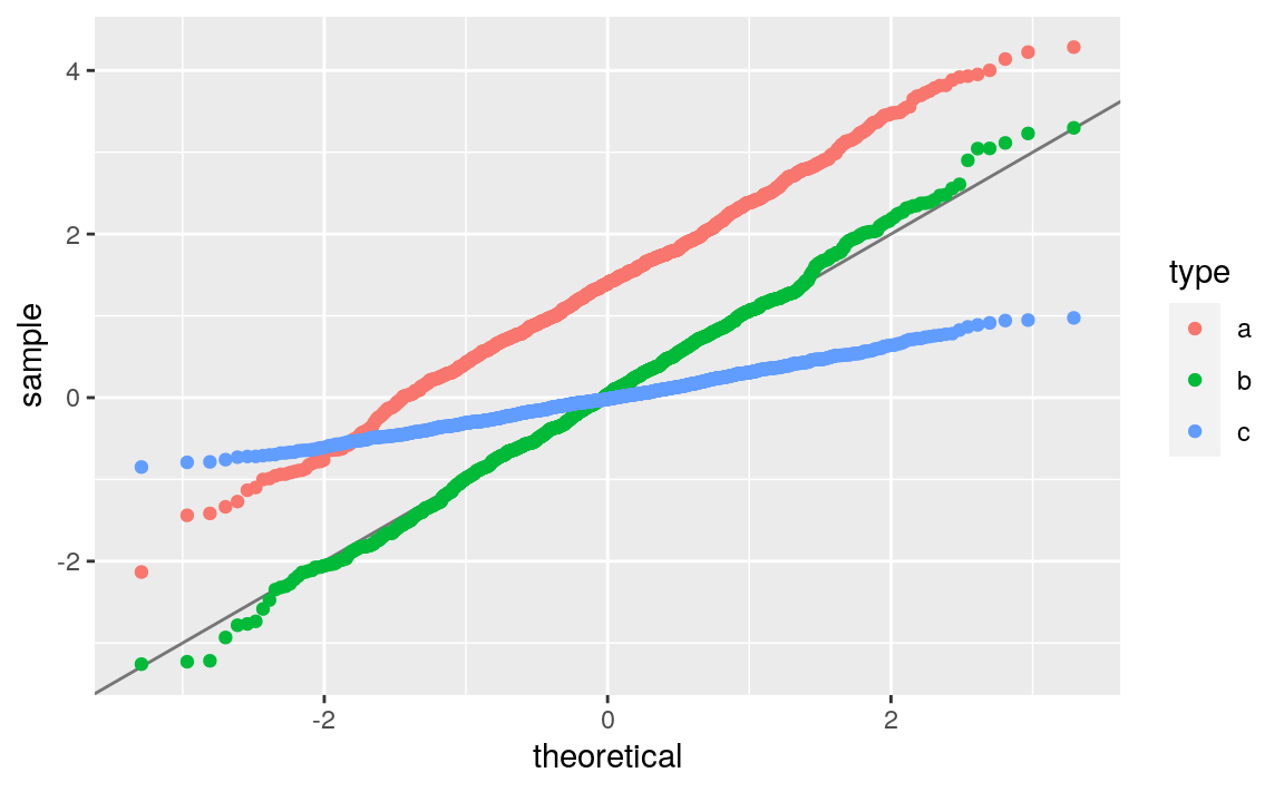

$Quantile-quantile plot of the standard normal law against the empirical laws of three estimators of $\psi_{0}$, one of them misconceived (a), one assuming that $\Gbar_{0}$ is known (b) and one that hinges on the estimation of $\Gbar_{0}$ (c). Built based on 1000 independent realizations of each estimator.$

Figure 8.2: Quantile-quantile plot of the standard normal law against the empirical laws of three estimators of $\psi_{0}$, one of them misconceived (a), one assuming that $\Gbar_{0}$ is known (b) and one that hinges on the estimation of $\Gbar_{0}$ (c). Built based on 1000 independent realizations of each estimator.

Figures 8.1 and 8.2 confirm that $\psi_{n}^{c}$ behaves almost as well as $\psi_{n}^{b}$ in terms of bias — but remember that we acted as oracles when we chose the well-specified algorithm $\Algo_{\Gbar,1}$. They also corroborate that $v_{n}^{c}$, the estimator of the asymptotic variance of $\sqrt{n} (\psi_{n}^{c} - \psi_{0})$, is conservative: for instance, the corresponding bell-shaped blue curve is too much concentrated around its axis of symmetry.

The actual asymptotic variance of $\sqrt{n} (\psi_{n}^{c} - \psi_{0})$ can be estimated with the empirical variance of the 1000 replications of the construction of $\psi_{n}^{c}$.

(emp_sig_n <- psi_hat_abc %>% filter(type == "c") %>%
   summarize(sd(psi_n)) %>% pull)
#> [1] 0.0172
(summ_sig_n <- psi_hat_abc %>% filter(type == "c") %>% select(sig_n) %>%
   summary)
#>      sig_n       
#>  Min.   :0.0517  
#>  1st Qu.:0.0549  
#>  Median :0.0559  
#>  Mean   :0.0560  
#>  3rd Qu.:0.0570  
#>  Max.   :0.0623

The empirical standard deviation is approximately 3.254 times smaller than the average estimated standard deviation. The estimator is conservative indeed! Furthermore, note the better fit with the density of the standard normal density of the kernel density estimator of the law of $\sqrt{n} (\psi_{n}^{c} - \psi_{0})$ renormalized with emp_sig_n.

clt_c <- psi_hat_abc %>% filter(type == "c") %>%
  mutate(clt = clt * sig_n / emp_sig_n)

fig_bias_ab +
  geom_density(aes(clt, fill = type, colour = type), clt_c, alpha = 0.1) +
  geom_vline(aes(xintercept = bias, colour = type),
             bias_abc, size = 1.5, alpha = 0.5) +
  xlim(-3, 4) + 
  labs(y = "",
       x = bquote(paste(sqrt(n/v[n]^{list(a, b, c)})*
                        (psi[n]^{list(a, b, c)} - psi[0]))))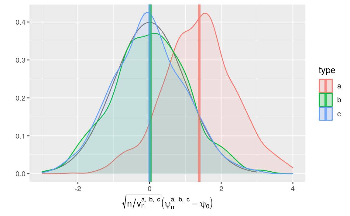

$Kernel density estimators of the law of three estimators of $\psi_{0}$ (recentered with respect to $\psi_{0}$, and renormalized), one of them misconceived (a), one assuming that $\Gbar_{0}$ is known (b) and one that hinges on the estimation of $\Gbar_{0}$ and an estimator of the asymptotic variance computed across the replications (c). The present figure includes Figure 6.1 (but the colors differ) and it should be compared to Figure 8.2. Built based on 1000 independent realizations of each estimator.$

Figure 8.3: Kernel density estimators of the law of three estimators of $\psi_{0}$ (recentered with respect to $\psi_{0}$, and renormalized), one of them misconceived (a), one assuming that $\Gbar_{0}$ is known (b) and one that hinges on the estimation of $\Gbar_{0}$ and an estimator of the asymptotic variance computed across the replications (c). The present figure includes Figure 6.1 (but the colors differ) and it should be compared to Figure 8.2. Built based on 1000 independent realizations of each estimator.

Workaround. In a real world data-analysis, one could correct the estimation of the asymptotic variance of $\sqrt{n} (\psi_{n}^{c} - \psi_{0})$. We could for instance derive the influence function as it is described there in Appendix C.1.1 and use the corresponding influence function-based estimator of the variance. One could also rely on the cross-validation, possibly combined with the previous workaround. Or one could also rely on the bootstrap.¹⁷ This, however, would only make sense if one knew for sure that the algorithm for the estimation of $\Gbar_{0}$ is well-specified.

8.3 ⚙ Investigating further the IPTW inference strategy

Building upon the chunks of code devoted to the repeated computation of $\psi_{n}^{b}$ and its companion quantities, construct confidence intervals for $\psi_{0}$ of (asymptotic) level $95\%$, and check if the empirical coverage is satisfactory. Note that if the coverage was exactly $95\%$, then the number of confidence intervals that would contain $\psi_{0}$ would follow a binomial law with parameters 1000 and 0.95, and recall that function binom.test performs an exact test of a simple null hypothesis about the probability of success in a Bernoulli experiment against its three one-sided and two-sided alternatives.
Discuss what happens when the dimension of the (still well-specified) working model grows. Start with the built-in working model working_model_G_two. The following chunk of code re-defines working_model_G_two

## make sure '1/2' and '1' belong to 'powers'
powers <- rep(seq(1/4, 3, by = 1/4), each = 2) 
working_model_G_two <- list(
  model = function(...) {trim_glm_fit(glm(family = binomial(), ...))},
  formula = stats::as.formula(
    paste("A ~",
          paste(c("I(W^", "I(abs(W - 5/12)^"),
                powers, 
                sep = "", collapse = ") + "),
          ")")
  ),
  type_of_preds = "response"
)
attr(working_model_G_two, "ML") <- FALSE

Play around with argument powers (making sure that 1/2 and 1 belong to it), and plot graphics similar to those presented in Figures 8.1 and 8.2.
Discuss what happens when the working model is mis-specified. You could use the built-in working model working_model_G_three.
Repeat the analysis developed in response to problem 1 above but for $\psi_{n}^{c}$. What can you say about the coverage of the confidence intervals?
☡ (Follow-up to problem 5). Implement the bootstrap procedure evoked at the end of Section 8.2.3. Repeat the analysis developed in response to problem 1. Compare your results with those to problem 5.
☡ Is it legitimate to infer the asymptotic variance of $\psi_{n}^{c}$ with $v_{n}^{c}$ when one relies on a very data-adaptive/versatile algorithm to estimate $\Gbar_{0}$?

8.4 G-computation estimator

8.4.1 Construction and computation

Let $\Algo_{Q_{W}}$ be an algorithm designed for the estimation of $Q_{0,W}$ (see Section 7.3). We denote by $Q_{n,W} \defq \Algo_{Q_{W}}(P_{n})$ the output of the algorithm trained on $P_{n}$.

Let $\Algo_{\Qbar}$ be an algorithm designed for the estimation of $\Qbar_{0}$ (see Section 7.6). We denote by $\Qbar_{n} \defq \Algo_{\Qbar}(P_{n})$ the output of the algorithm trained on $P_{n}$.

Equation (2.1) suggests the following, simple estimator of $\Psi(P_0)$:

\[\begin{equation} \psi_{n} \defq \int \left(\Qbar_{n}(1, w) - \Qbar_{n}(0,w)\right) dQ_{n,W}(w). \tag{8.1} \end{equation}\]

In words, this estimator is implemented by first regressing $Y$ on $(A,W)$, then by marginalizing with respect to the estimated law of $W$. The resulting estimator is referred to as a G-computation (or standardization) estimator.

From a computational point of view, the tlrider package makes it easy to build the G-computation estimator. Recall that we have already estimated the marginal law $Q_{0,W}$ of $W$ under $P_{0}$ by training the algorithm $\Algo_{Q_{W}}$ as it is implemented in estimate_QW on the $n = 1000$ first observations in obs (see Section 7.3):

QW_hat <- estimate_QW(head(obs, 1e3))

Recall that $\Algo_{\Qbar,1}$ is the algorithm for the estimation of $\Qbar_{0}$ as it is implemented in estimate_Qbar with its argument algorithm set to the built-in working_model_Q_one (see Section 7.5). Recall also that $\Algo_{\Qbar,\text{kNN}}$ is the algorithm for the estimation of $\Qbar_{0}$ as it is implemented in estimate_Qbar with its argument algorithm set to the built-in kknn_algo (see Section 7.6.2). We have already trained the latter on the $n=1000$ first observations in obs. Let us train the former on the same data set:

Qbar_hat_kknn <- estimate_Qbar(head(obs, 1e3),
                               algorithm = kknn_algo,
                               trControl = kknn_control,
                               tuneGrid = kknn_grid)

Qbar_hat_d <- estimate_Qbar(head(obs, 1e3), working_model_Q_one)

With these estimators handy, computing the G-computation estimator is as simple as running the following chunk of code:

(compute_gcomp(QW_hat, wrapper(Qbar_hat_kknn, FALSE), 1e3))
#> # A tibble: 1 × 2
#>   psi_n   sig_n
#>   <dbl>   <dbl>
#> 1 0.101 0.00306
(compute_gcomp(QW_hat, wrapper(Qbar_hat_d, FALSE), 1e3))
#> # A tibble: 1 × 2
#>   psi_n   sig_n
#>   <dbl>   <dbl>
#> 1 0.109 0.00215

Note how we use function wrapper again, and that it is necessary to provide the number of observations upon which the estimation of the $Q_{W}$ and $\Qbar$ features of $P_{0}$.

8.4.2 Elementary statistical properties

This subsection is very similar to its counterpart for the IPTW estimator, see Section 8.2.2.

Let us denote by $\Qbar_{n,1}$ the output of algorithm $\Algo_{\Qbar,1}$ trained on $P_{n}$, and recall that $\Qbar_{n,\text{kNN}}$ is the output of algorithm $\Algo_{\Qbar,\text{kNN}}$ trained on $P_{n}$. Let $\psi_{n}^{d}$ and $\psi_{n}^{e}$ be the G-computation estimators obtained by substituting $\Qbar_{n,1}$ and $\Qbar_{n,\text{kNN}}$ for $\Qbar_{n}$ in (8.1), respectively.

If $\Qbar_{n,\bullet}$ minimized the empirical risk over a finite-dimensional, identifiable, and well-specified working model, then $\sqrt{n} (\psi_{n}^{\bullet} - \psi_{0})$ would converge in law to a centered Gaussian law (here $\psi_{n}^{\bullet}$ represents the G-computation estimator obtained by substituting $\Qbar_{n,\bullet}$ for $\Qbar_{n}$ in (8.1)). Moreover, the asymptotic variance of $\sqrt{n} (\psi_{n}^{\bullet} - \psi_{0})$ would be estimated anti-conservatively¹⁸ with

\[\begin{align} v_{n}^{d} &\defq \Var_{P_{n}} \left(\Qbar_{n,1}(1,\cdot) - \Qbar_{n,1}(0,\cdot)\right) \\ &= \frac{1}{n} \sum_{i=1}^{n}\left(\Qbar_{n,1}(1,W_{i}) - \Qbar_{n,1}(0,W_{i}) -\psi_{n}^{d}\right)^{2}. \tag{8.2} \end{align}\]

Unfortunately, algorithm $\Algo_{\Qbar,1}$ is mis-specified and $\Algo_{\Qbar,\text{kNN}}$ is not based on a finite-dimensional working model. Nevertheless, function compute_gcomp estimates (in general, very poorly) the asymptotic variance with (8.2).

We investigate empirically the statistical behavior of $\psi_{n}^{d}$ in Section 8.4.3. For an analysis of the reason why $v_{n}^{d}$ is an anti-conservative estimator of the asymptotic variance of $\sqrt{n} (\psi_{n}^{d} - \psi_{0})$, see there in Appendix C.1.2. We wish to emphasize that anti-conservativeness is even more embarrassing that conservativeness (both being contingent on the fact that the algorithms are well-specified, fact that cannot be true in the present case in real world situations).

What would happen if we used a less amenable algorithm $\Algo_{\Qbar}$. For instance, $\Algo_{\Qbar}$ could still be well-specified but so versatile/complex (as opposed to being based on well-behaved, finite-dimensional parametric model) that the estimator $\Qbar_{n}$, though still consistent, would converge slowly to its target. Then, root-$n$ consistency would fail to hold. We can explore empirically this situation with estimator $\psi_{n}^{e}$ that hinges on algorithm $\Algo_{\Qbar,\text{kNN}}$. Or $\Algo_{\Qbar}$ could be mis-specified and there would be no guarantee at all that the resulting estimator $\psi_{n}$ be even consistent.

8.4.3 Empirical investigation, fixed sample size

Let us compute $\psi_{n}^{d}$ and $\psi_{n}^{e}$ on the same iter = 1000 independent samples of independent observations drawn from $P_{0}$ as in Sections 6.3 and 8.2.3. We first enrich object learned_features_fixed_sample_size that was created in Section 8.2.3, adding to it estimators of $\Qbar_{0}$ obtained by training algorithms $\Algo_{\Qbar,1}$ and $\Algo_{\Qbar,\text{kNN}}$ on each smaller data set.

The second series of commands creates object psi_hat_de, an 1000 by six tibble containing notably the values of $\psi_{n}^{d}$ and $\sqrt{v_{n}^{d}}/\sqrt{n}$ computed by calling compute_gcomp, and those of the recentered (with respect to $\psi_{0}$) and renormalized $\sqrt{n}/\sqrt{v_{n}^{d}} (\psi_{n}^{d} - \psi_{0})$. Because we know beforehand that $v_{n}^{d}$ under-estimates the actual asymptotic variance of $\sqrt{n} (\psi_{n}^{d} - \psi_{0})$, the tibble also includes the values of $\sqrt{n}/\sqrt{v^{d*}} (\psi_{n}^{d} - \psi_{0})$ where the estimator $v^{d*}$ of the asymptotic variance is computed across the replications of $\psi_{n}^{d}$. The tibble includes the same quantities pertaining to $\psi_{n}^{e}$, although there is no theoretical guarantee that the central limit theorem does hold and, even if it did, that the counterpart $v_{n}^{e}$ to $v_{n}^{d}$ estimates in any way the asymptotic variance of $\sqrt{n} (\psi_{n}^{e} - \psi_{0})$.

Finally, bias_de reports amounts of bias (at the renormalized scales — plural). There is one value of bias for each combination of (i) type of the estimator (d or e) and (ii) how the renormalization is carried out, either based on $v_{n}^{d}$ and $v_{n}^{e}$ (auto_renormalization is TRUE) or on the estimator of the asymptotic variance computed across the replications of $\psi_{n}^{d}$ and $\psi_{n}^{e}$ (auto_renormalization is FALSE).

learned_features_fixed_sample_size <-
  learned_features_fixed_sample_size %>% 
  mutate(Qbar_hat_d =
           map(obs,
               ~ estimate_Qbar(., algorithm = working_model_Q_one)),
         Qbar_hat_e =
           map(obs,
               ~ estimate_Qbar(., algorithm = kknn_algo,
                               trControl = kknn_control,
                               tuneGrid = kknn_grid))) %>%
  mutate(QW = map(obs, estimate_QW),
         est_d =
           pmap(list(QW, Qbar_hat_d, n()),
                ~ compute_gcomp(..1, wrapper(..2, FALSE), ..3)),
         est_e =
           pmap(list(QW, Qbar_hat_e, n()),
                ~ compute_gcomp(..1, wrapper(..2, FALSE), ..3)))

psi_hat_de <- learned_features_fixed_sample_size %>%
  select(est_d, est_e) %>%
  pivot_longer(c(`est_d`, `est_e`),
               names_to = "type", values_to = "estimates") %>%
  extract(type, "type", "_([de])$") %>% 
  unnest(estimates) %>%
  group_by(type) %>%
  mutate(sig_alt = sd(psi_n)) %>%
  mutate(clt_ = (psi_n - psi_zero) / sig_n,
         clt_alt = (psi_n - psi_zero) / sig_alt) %>%
  pivot_longer(c(`clt_`, `clt_alt`),
               names_to = "key", values_to = "clt") %>%
  extract(key, "key", "_(.*)$") %>%
  mutate(key = ifelse(key == "", TRUE, FALSE)) %>%
  rename("auto_renormalization" = key)

(bias_de <- psi_hat_de %>%
   group_by(type, auto_renormalization) %>%
   summarize(bias = mean(clt), .groups = "drop"))
#> # A tibble: 4 × 3
#>   type  auto_renormalization  bias
#>   <chr> <lgl>                <dbl>
#> 1 d     FALSE                0.234
#> 2 d     TRUE                 2.04 
#> 3 e     FALSE                0.107
#> 4 e     TRUE                 0.626

fig <- ggplot() +
  geom_line(aes(x = x, y = y), 
            data = tibble(x = seq(-4, 4, length.out = 1e3),
                          y = dnorm(x)),
            linetype = 1, alpha = 0.5) +
  geom_density(aes(clt, fill = type, colour = type),
               psi_hat_de, alpha = 0.1) +
  geom_vline(aes(xintercept = bias, colour = type),
             bias_de, size = 1.5, alpha = 0.5) +
  facet_wrap(~ auto_renormalization,
             labeller =
               as_labeller(c(`TRUE` = "auto-renormalization: TRUE",
                             `FALSE` = "auto-renormalization: FALSE")),
             scales = "free")
  
fig +
  labs(y = "",
       x = bquote(paste(sqrt(n/v[n]^{list(d, e)})*
                        (psi[n]^{list(d, e)} - psi[0]))))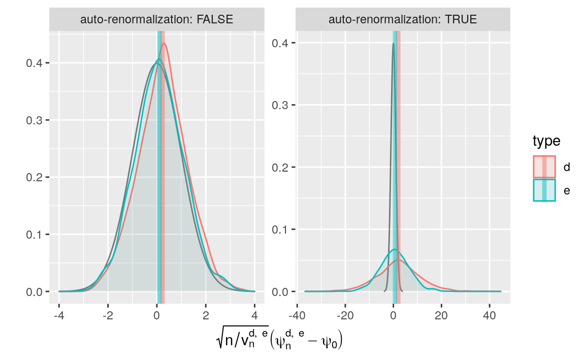

$Kernel density estimators of the law of two G-computation estimators of $\psi_{0}$ (recentered with respect to $\psi_{0}$, and renormalized). The estimators respectively hinge on algorithms $\Algo_{\Qbar,1}$ (d) and $\Algo_{\Qbar,\text{kNN}}$ (e) to estimate $\Qbar_{0}$. Two renormalization schemes are considered, either based on an estimator of the asymptotic variance (right) or on the empirical variance computed across the 1000 independent replications of the estimators (left). We emphasize that the $x$-axis ranges differ between the left and right plots.$

Figure 8.4: Kernel density estimators of the law of two G-computation estimators of $\psi_{0}$ (recentered with respect to $\psi_{0}$, and renormalized). The estimators respectively hinge on algorithms $\Algo_{\Qbar,1}$ (d) and $\Algo_{\Qbar,\text{kNN}}$ (e) to estimate $\Qbar_{0}$. Two renormalization schemes are considered, either based on an estimator of the asymptotic variance (right) or on the empirical variance computed across the 1000 independent replications of the estimators (left). We emphasize that the $x$-axis ranges differ between the left and right plots.

We represent the empirical laws of the recentered (with respect to $\psi_{0}$) and renormalized $\psi_{n}^{d}$ and $\psi_{n}^{e}$ in Figure 8.4 (kernel density estimators). Two renormalization schemes are considered, either based on an estimator of the asymptotic variance (left) or on the empirical variance computed across the 1000 independent replications of the estimators (right). We emphasize that the $x$-axis ranges differ between the left and right plots.

Two important comments are in order. First, on the one hand, the G-computation estimator $\psi_{n}^{d}$ is biased. Specifically, by the above chunk of code, the averages of $\sqrt{n/v_{n}^{d}} (\psi_{n}^{d} - \psi_{0})$ and $\sqrt{n/v_{n}^{d*}} (\psi_{n}^{d} - \psi_{0})$ computed across the realizations are equal to 2.038 and 0.234 (see bias_de). On the other hand, the G-computation estimator $\psi_{n}^{e}$ is biased too, though slightly less than $\psi_{n}^{d}$. Specifically, by the above chunk of code, the averages of $\sqrt{n/v_{n}^{e}} (\psi_{n}^{e} - \psi_{0})$ and $\sqrt{n/v^{e*}} (\psi_{n}^{e} - \psi_{0})$ computed across the realizations are equal to 0.626 and 0.107 (see bias_de). We can provide an oracular explanation. Estimator $\psi_{n}^{d}$ suffers from the poor approximation of $\Qbar_{0}$ by $\Algo_{\Qbar,1}(P_{n})$, a result of the algorithm’s mis-specification. As for $\psi_{n}^{e}$, it behaves better because $\Algo_{\Qbar,\text{kNN}} (P_{n})$ approximates $\Qbar_{0}$ better than $\Algo_{\Qbar,1}(P_{n})$, an apparent consequence of the greater versatility of the algorithm.

Second, we get a visual confirmation that $v_{n}^{d}$ under-estimates the actual asymptotic variance of $\sqrt{n} (\psi_{n}^{d} - \psi_{0})$: the right-hand side red bell-shaped curve is too dispersed. In contrast, the right-hand side blue bell-shaped curve is much closer to the black curve that represents the density of the standard normal law. Looking at the left-hand side plot reveals that the empirical law of $\sqrt{n/v^{d*}} (\psi_{n}^{d} - \psi_{0})$, once translated to compensate for the bias, is rather close to the black curve. This means that the random variable is approximately distributed like a Gaussian random variable. On the contrary, the empirical law of $\sqrt{n/v^{e*}} (\psi_{n}^{e} - \psi_{0})$ does not strike us as being as closely Gaussian-like as that of $\sqrt{n/v^{d*}} (\psi_{n}^{d} - \psi_{0})$. By being more data-adaptive than $\Algo_{\Qbar,1}$, algorithm $\Algo_{\Qbar,\text{kNN}}$ yields a better estimator of $\Qbar_{0}$. However, the rate of convergence of $\Algo_{\Qbar,\text{kNN}}(P_{n})$ to its limit may be slower than root-$n$, invalidating a central limit theorem.

How do the estimated variances of $\psi_{n}^{d}$ and $\psi_{n}^{e}$ compare with their empirical counterparts (computed across the 1000 replications of the construction of the two estimators)?

## psi_n^d
(psi_hat_de %>% ungroup %>%
   filter(type == "d" & auto_renormalization) %>% pull(sig_n) %>% summary)
#>    Min. 1st Qu.  Median    Mean 3rd Qu.    Max. 
#> 0.00019 0.00169 0.00205 0.00206 0.00241 0.00369
## psi_n^e
(psi_hat_de %>% ungroup %>%
   filter(type == "e" & auto_renormalization) %>% pull(sig_n) %>% summary)
#>    Min. 1st Qu.  Median    Mean 3rd Qu.    Max. 
#> 0.00170 0.00261 0.00287 0.00288 0.00314 0.00421

The empirical standard deviation of $\psi_{n}^{d}$ is approximately 8.307 times larger than the average estimated standard deviation. The estimator is anti-conservative indeed!

As for the empirical standard deviation of $\psi_{n}^{e}$, it is approximately 5.962 times larger than the average estimated standard deviation.

8.4.4 ☡ Empirical investigation, varying sample size

sample_size <- c(2500, 5000) # 5e3, 15e3
block_size <- sum(sample_size)


learned_features_varying_sample_size <- obs %>% as_tibble %>% 
  head(n = (nrow(.) %/% block_size) * block_size) %>% 
  mutate(block = label(1:nrow(.), sample_size)) %>%
  nest(obs = c(W, A, Y))

First, we cut the data set into independent sub-data sets of sample size $n$ in $\{$ 2500, 5000 $\}$. Second, we infer $\psi_{0}$ as shown two chunks earlier. We thus obtain 133 independent realizations of each estimator derived on data sets of r length(sample_size), increasing sample sizes.

learned_features_varying_sample_size <-
  learned_features_varying_sample_size %>%
  mutate(Qbar_hat_d =
           map(obs,
               ~ estimate_Qbar(., algorithm = working_model_Q_one)),
         Qbar_hat_e =
           map(obs,
               ~ estimate_Qbar(., algorithm = kknn_algo,
                               trControl = kknn_control,
                               tuneGrid = kknn_grid))) %>%
  mutate(QW = map(obs, estimate_QW),
         est_d =
           pmap(list(QW, Qbar_hat_d, n()),
                ~ compute_gcomp(..1, wrapper(..2, FALSE), ..3)),
         est_e =
           pmap(list(QW, Qbar_hat_e, n()),
                ~ compute_gcomp(..1, wrapper(..2, FALSE), ..3)))

root_n_bias <- learned_features_varying_sample_size %>%
  mutate(block = unlist(map(strsplit(block, "_"), ~.x[2])),
         sample_size = sample_size[as.integer(block)]) %>%
  select(block, sample_size, est_d, est_e) %>%
  pivot_longer(c(`est_d`, `est_e`),
               names_to = "type", values_to = "estimates") %>%
  extract(type, "type", "_([de])$") %>% 
  unnest(estimates) %>%
  group_by(block, type) %>%
  mutate(sig_alt = sd(psi_n)) %>%
  mutate(clt_ = (psi_n - psi_zero) / sig_n,
         clt_alt = (psi_n - psi_zero) / sig_alt) %>%
  pivot_longer(c(`clt_`, `clt_alt`),
               names_to = "key", values_to = "clt") %>%
  extract(key, "key", "_(.*)$") %>%
  mutate(key = ifelse(key == "", TRUE, FALSE)) %>%
  rename("auto_renormalization" = key)

The tibble called root_n_bias reports root-$n$ times bias for all combinations of estimator and sample size. The next chunk of code presents visually our findings, see Figure 8.5. Note how we include the realizations of the estimators derived earlier and contained in psi_hat_de (thus breaking the independence between components of root_n_bias, a small price to pay in this context).

root_n_bias <- learned_features_fixed_sample_size %>%
   mutate(block = "0",
          sample_size = B/iter) %>%  # because *fixed* sample size
   select(block, sample_size, est_d, est_e) %>%
  pivot_longer(c(`est_d`, `est_e`),
               names_to = "type", values_to = "estimates") %>%
   extract(type, "type", "_([de])$") %>% 
   unnest(estimates) %>%
   group_by(block, type) %>%
   mutate(sig_alt = sd(psi_n)) %>%
   mutate(clt_ = (psi_n - psi_zero) / sig_n,
          clt_alt = (psi_n - psi_zero) / sig_alt) %>%
  pivot_longer(c(`clt_`, `clt_alt`),
               names_to = "key", values_to = "clt") %>%
   extract(key, "key", "_(.*)$") %>%
   mutate(key = ifelse(key == "", TRUE, FALSE)) %>%
   rename("auto_renormalization" = key) %>%
   full_join(root_n_bias)
 
root_n_bias %>% filter(auto_renormalization) %>%
  mutate(rnb = sqrt(sample_size) * (psi_n - psi_zero)) %>%
  group_by(sample_size, type) %>%
  ggplot() +
  stat_summary(aes(x = sample_size, y = rnb,
                   group = interaction(sample_size, type),
                   color = type),
               fun.data = mean_se, fun.args = list(mult = 1),
               position = position_dodge(width = 250), cex = 1) +
  stat_summary(aes(x = sample_size, y = rnb,
                   group = interaction(sample_size, type),
                   color = type),
               fun.data = mean_se, fun.args = list(mult = 1),
               position = position_dodge(width = 250), cex = 1,
               geom = "errorbar", width = 750) +
  stat_summary(aes(x = sample_size, y = rnb,
                   color = type),
               fun = mean,
               position = position_dodge(width = 250),
               geom = "polygon", fill = NA) +
  geom_point(aes(x = sample_size, y = rnb,
                 group = interaction(sample_size, type),
                 color = type),
             position = position_dodge(width = 250),
             alpha = 0.1) +
  scale_x_continuous(breaks = unique(c(B / iter, sample_size))) +
  labs(x = "sample size n",
       y = bquote(paste(sqrt(n) * (psi[n]^{list(d, e)} - psi[0]))))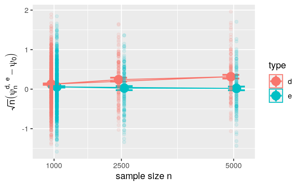

$Evolution of root-$n$ times bias versus sample size for two G-computation estimators of $\psi_{0}$. The estimators respectively hinge on algorithms $\Algo_{\Qbar,1}$ (d) and $\Algo_{\Qbar,\text{kNN}}$ (e) to estimate $\Qbar_{0}$. Big dots represent the average biases and vertical lines represent twice the standard error.$

Figure 8.5: Evolution of root-$n$ times bias versus sample size for two G-computation estimators of $\psi_{0}$. The estimators respectively hinge on algorithms $\Algo_{\Qbar,1}$ (d) and $\Algo_{\Qbar,\text{kNN}}$ (e) to estimate $\Qbar_{0}$. Big dots represent the average biases and vertical lines represent twice the standard error.

On the one hand, root-$n$ bias for $\psi_{n}^{e}$ tends to decrease from sample size 1000 to 5000 where it tends to be small in average.¹⁹ On the other hand, root-$n$ bias for $\psi_{n}^{d}$ (red lines and points) is positive and tends to increase from sample size 1000 to 2500 and from 2500 to 5000. Overall, root-$n$ bias tends to be larger for $\psi_{n}^{d}$ than for $\psi_{n}^{e}$.

In essence, we observe that the bias does not vanish faster than root-$n$. For $\psi_{n}^{d}$, this is because $\Algo_{\Qbar,1}$ is mis-specified and we expect that the bias increases at rate root-$n$. For $\psi_{n}^{e}$, this is because the estimator produced by the versatile $\Algo_{\Qbar,\text{kNN}}$ converges slowly to its limit. Can anything be done to amend $\psi_{n}^{d}$ and $\psi_{n}^{e}$?

8.5 ⚙ Investigating further the G-computation estimation strategy

Implement the G-computation estimator based on well-specified working model. To do so, (i) create a copy working_model_Q_two of working_model_Q_one, (ii) replace its family entry in such a way that $\Qbar_{0}$ falls in the corresponding working model, and (iii) adapt the chunk of code where we computed Qbar_hat_d in Section 8.4.1.
Evaluate the empirical properties of the estimator of problem 1.
Create a function to estimate the marginal law $Q_{0,W}$ of $W$ by maximum likelihood estimation based on a mis-specified model that assumes (wrongly) that $W$ is drawn from a Gaussian law with unknown mean and variance.
☡ Implement the G-computation estimator using either working_model_Q_one or working_model_Q_two and the estimator of $Q_{0,W}$ of problem 3.

In words, $v_{n}^{c}$ converges to an upper-bound of the true asymptotic variance.↩︎
Well-specified e.g. in the sense that the target $\Gbar_{0}$ of $\Algo_{\Gbar}$ belongs to the closure of the algorithm’s image $\Algo_{\Gbar}(\calM^{\text{empirical}})$ or, in other words, can be approximated arbitrarily well by an output of the algorithm.↩︎
That is, replicate the construction of $\psi_{n}^{c}$ many times based on data sets obtained by resampling from the original data set, then estimate the asymptotic variance with the empirical variance of $\psi_{n}^{c}$ computed across the replications.↩︎
In words, $v_{n}^{d}$ converges to a lower-bound of the true asymptotic variance.↩︎
We use the expression ``tend to be’’ because controlling for multiple testing makes it impossible to make a firm statement.↩︎