Section 7 Nuisance parameters
7.1 Anatomy of an expression
From now, all the inference strategies that we will present unfold in two or three stages. For all of them, the first stage consists in estimating a selection of features of the law \(P_{0}\) of the experiment. Specifically, the features are chosen among \(Q_{0,W}\) (the marginal law of \(W\) under \(P_{0}\)), \(\Gbar_{0}\) (the conditional probability that \(A=1\) given \(W\) under \(P_{0}\)) and \(\Qbar_{0}\) (the conditional mean of \(Y\) given \(A\) and \(W\) under \(P_{0}\)).
In this context, because they are not the parameter of primary interest (i.e., they are not the real-valued feature \(\Psi(P_{0})\)), they are often referred to as nuisance parameters of \(P_{0}\). The unflaterring expression conveys the notion that their estimation is merely an intermediate step along our path towards an inference of the target parameter.
As for the reason why \(Q_{0,W}\), \(\Gbar_{0}\) and \(\Qbar_{0}\) are singled out, it is because of their role in the definition of \(\Psi\) and the efficient influence curve \(D^{*}(P_{0})\).
7.2 An algorithmic stance
In general, we can view an estimator of any feature \(f_0\) of \(P_{0}\) as the output of an algorithm \(\Algo\) that maps any element of
\[\begin{equation*} \calM^{\text{empirical}} \defq \left\{\frac{1}{m} \sum_{i=1}^{m} \Dirac(o_{i}) : m \geq 1, o_{1}, \ldots, o_{m} \in [0,1] \times \{0,1\} \times [0,1]\right\} \end{equation*}\]
to the set \(\calF\) where \(f_{0}\) is known to live. Here, \(\calM^{\text{empirical}}\) can be interpreted as the set of all possible empirical measures summarizing the outcomes of any number of replications of the experiment \(P_{0}\). In particular, \(P_{n}\) belongs to this set.
The tlrider package includes such template algorithms for the estimation of
\(Q_{0,W}\), \(\Gbar_{0}\) and \(\Qbar_{0}\). We illustrate how they work and their
use in the next sections.
7.3 QW
For instance, estimate_QW is an algorithm \(\Algo_{Q_{W}}\) for the estimation
of the marginal law of \(W\) under \(P_{0}\) (to see its man page, simply run
?estimate_QW). It is a map from \(\calM^{\text{empirical}}\) to the set of
laws on \([0,1]\). The following chunk of code estimates \(Q_{0,W}\) based on the
\(n = 1000\) first observations in obs:
QW_hat <- estimate_QW(head(obs, 1e3))It is easy to sample independent observations from QW_hat. To do so, we
create an object of class LAW then set its marginal law of \(W\) to that
described by QW_hat and specify its sample_from feature:
empirical_experiment <- LAW()
alter(empirical_experiment, QW = QW_hat)
alter(empirical_experiment, sample_from = function(n) {
  QW <- get_feature(empirical_experiment, "QW")
  W <- sample(pull(QW, "value"), n, prob = pull(QW, "weight"))
  cbind(W = W, A = NA, Y = NA)
})
W <- sample_from(empirical_experiment, 1e3) %>% as_tibble

W %>%
ggplot() +
  geom_histogram(aes(x = W, y = stat(density)), bins = 40) +
  stat_function(fun = get_feature(experiment, "QW"), col = "red")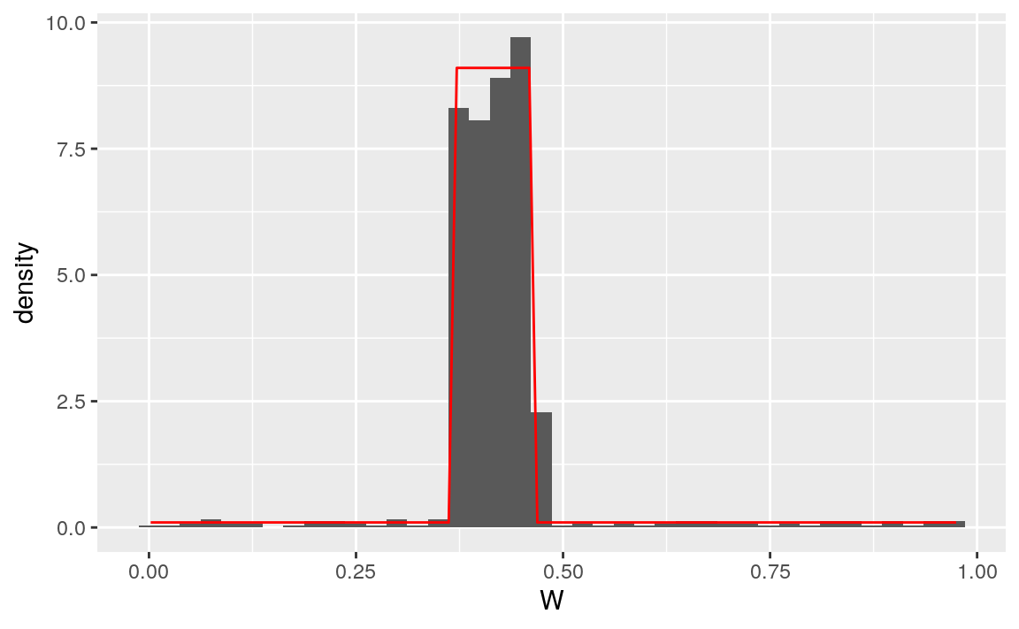
Figure 7.1: Histogram representing 1000 observations drawn independently from QW_hat. The superimposed red curve is the true density of \(Q_{0,W}\).
Note that all the \(W\)s sampled from QW_hat fall in the set \(\{W_{1}, \ldots, W_{n}\}\) of observed \(W\)s in obs (an obvious fact given the definition of
the sample_from feature of empirical_experiment:
(length(intersect(pull(W, W), head(obs[, "W"], 1e3))))
#> [1] 1000
This is because estimate_QW estimates \(Q_{0,W}\) with its empirical
counterpart, i.e.,
\[\begin{equation*}\frac{1}{n} \sum_{i=1}^{n} \Dirac(W_{i}).\end{equation*}\]
7.4 Gbar
Another template algorithm is built-in into tlrider: estimate_Gbar (to see
its man page, simply run ?estimate_Gbar). Unlike estimate_QW,
estimate_Gbar needs further specification of the algorithm. The package also
includes examples of such specifications.
There are two sorts of specifications, of which we say that they are either working model-based or machine learning-based. We discuss the former sort in the next subsection. The latter sort is discussed in Section 7.6.
7.4.1 Working model-based algorithms
Let us take a look at working_model_G_one for instance:
working_model_G_one
#> $model
#> function (...)
#> {
#>     trim_glm_fit(glm(family = binomial(), ...))
#> }
#> <environment: 0x56115606af08>
#>
#> $formula
#> A ~ I(W^0.5) + I(abs(W - 5/12)^0.5) + I(W^1) + I(abs(W - 5/12)^1) +
#>     I(W^1.5) + I(abs(W - 5/12)^1.5)
#> <environment: 0x56115606af08>
#>
#> $type_of_preds
#> [1] "response"
#>
#> attr(,"ML")
#> [1] FALSE
and focus on its model and formula attributes. The former relies on the
glm and binomial functions from base R, and on trim_glm_fit (which
removes information that we do not need from the standard output of glm,
simply run ?trim_glm_fit to see the function’s man page). The latter is a
formula that characterizes what we call a working model for \(\Gbar_{0}\).
In words, by using working_model_G_one we implicitly choose the so-called
logistic (or negative binomial) loss function \(L_{a}\) given by
\[\begin{equation} \tag{7.1} -L_{a}(f)(A,W) \defq A \log f(W) + (1 - A) \log (1 - f(W)) \end{equation}\]
for any function \(f : [0,1] \to [0,1]\) paired with the working model \[\begin{equation*} \calF_{1} \defq \left\{f_{\theta} : \theta \in \bbR^{7}\right\} \end{equation*}\] where, for any \(\theta \in \bbR^{7}\), \[\begin{equation*}\logit f_{\theta} (W) \defq \theta_{0} + \sum_{j=1}^{3} \left(\theta_{j} W^{j/2} + \theta_{3+j} |W - 5/12|^{j/2}\right).\end{equation*}\]
We acted as oracles when we specified the working model: it is well-specified, i.e., it happens that \(\Gbar_{0}\) is the unique minimizer of the risk entailed by \(L_{a}\) over \(\calF_{1}\): \[\begin{equation*}\Gbar_{0} = \mathop{\arg\min}_{f_{\theta} \in \calF_{1}} \Exp_{P_{0}} \left(L_{a}(f_{\theta})(A,W)\right).\end{equation*}\] Therefore, the estimator \(\Gbar_{n}\) obtained by minimizing the empirical risk
\[\begin{equation*} \Exp_{P_{n}} \left(L_{a}(f_{\theta})(A,W)\right) = \frac{1}{n} \sum_{i=1}^{n} L_{a}(f_{\theta})(A_{i},W_{i}) \end{equation*}\]
over \(\calF_{1}\) estimates \(\Gbar_{0}\) consistently.
Of course, it is seldom certain in real life that the target feature, here \(\Gbar_{0}\), belongs to the working model.11 Suppose for instance that we choose a small finite-dimensional working model \(\calF_{2}\) without acting as an oracle. Then consistency certainly fails to hold. However, if \(\Gbar_{0}\) can nevertheless be projected unambiguously onto \(\calF_{2}\) (an assumption that cannot be checked), then the estimator might converge to the projection.
7.4.2 Visualization
To illustrate the use of the algorithm \(\Algo_{\Gbar,1}\) obtained by combining
estimate_Gbar and working_model_G_one, let us estimate \(\Gbar_{0}\) based
on the first \(n = 1000\) observations in obs:
Gbar_hat <- estimate_Gbar(head(obs, 1e3), algorithm = working_model_G_one)Using compute_Gbar_hat_W12
(simply run ?compute_Gbar_hat_W to see its man page) makes it is easy to
compare visually the estimator \(\Gbar_{n} \defq \Algo_{\Gbar,1}(P_{n})\) with
its target \(\Gbar_0\):
tibble(w = seq(0, 1, length.out = 1e3)) %>%
  mutate("truth" = Gbar(w),
         "estimated" = compute_Gbar_hatW(w, Gbar_hat)) %>%
  pivot_longer(-w, names_to = "f", values_to = "value") %>%
  ggplot() +
  geom_line(aes(x = w, y = value, color = f), size = 1) +
  labs(y = "f(w)",
       title = bquote("Visualizing" ~ bar(G)[0] ~ "and" ~ hat(G)[n])) +
  ylim(NA, 1)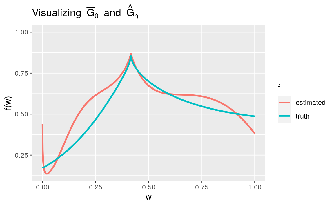
Figure 7.2: Comparing \(\Gbar_{n}\defq \Algo_{\Gbar,1}(P_{n})\) and \(\Gbar_{0}\). The estimator is consistent because the algorithm relies on a working model that is correctly specified.
7.5 ⚙ Qbar, working model-based algorithms
A third template algorithm is built-in into tlrider: estimate_Qbar (to see
its man page, simply run ?estimate_Qbar). Like estimate_Gbar,
estimate_Qbar needs further specification of the algorithm. The package also
includes examples of such specifications, which can also be either working
model-based (see Section 7.4) or machine learning-based (see
Sections 7.6 and 7.7).
There are built-in specifications similar to working_model_G_one, e.g.,
working_model_Q_one
#> $model
#> function (...)
#> {
#>     trim_glm_fit(glm(family = binomial(), ...))
#> }
#> <environment: 0x56115606af08>
#>
#> $formula
#> Y ~ A * (I(W^0.5) + I(W^1) + I(W^1.5))
#> <environment: 0x56115606af08>
#>
#> $type_of_preds
#> [1] "response"
#>
#> attr(,"ML")
#> [1] FALSE
#> attr(,"stratify")
#> [1] FALSE- Drawing inspiration from Section 7.4, comment upon and use
the algorithm \(\Algo_{\Qbar,1}\) obtained by combining
estimate_Gbarandworking_model_Q_one.
7.6 Qbar
7.6.1 Qbar, machine learning-based algorithms
We explained how algorithm \(\Algo_{\Gbar,1}\) is based on a working model (and you did for \(\Algo_{\Qbar,1}\)). It is not the case that all algorithms are based on working models in the same (admittedly rather narrow) sense. We propose to say that those algorithms that are not based on working models like \(\Algo_{\Gbar,1}\), for instance, are instead machine learning-based.
Typically, machine learning-based algorithms are more data-adaptive; they rely on larger working models, and/or fine-tune parameters that must be calibrated, e.g. by cross-validation. Furthermore, they call for being stacked, i.e., combined by means of another outer algorithm (involving cross-validation) into a more powerful machine learning-based meta-algorithm. The super learning methodology is a popular stacking algorithm.
We will elaborate further on this important topic in another forthcoming part
and merely touch upon it in Section 7.8. Here, we simply
illustrate the concept with two specifications built-in into tlrider. Based
on the \(k\)-nearest neighbors non-parametric estimating methodology, the
first one is discussed in the next subsection. Based on boosted trees,
another non-parametric estimating methodology, the second one is used in the
exercise that follows the next subsection.
7.6.2 Qbar, kNN algorithm
Algorithm \(\Algo_{\Qbar,\text{kNN}}\) is obtained by combining estimate_Qbar
and kknn_algo. The training of \(\Algo_{\Qbar,\text{kNN}}\) (i.e., the
making of the output \(\Algo_{\Qbar,\text{kNN}} (P_{n})\) is implemented based
on function caret::train of the caret (classification and regression
training) package (to see its man page, simply run ?caret::train). Some
additional specifications are provided in kknn_grid and kknn_control.
In a nutshell, \(\Algo_{\Qbar,\text{kNN}}\) estimates \(\Qbar_{0}(1,\cdot)\) and
\(\Qbar_{0}(0,\cdot)\) separately. Each of them is estimated by applying the
\(k\)-nearest neighbors methodology as it is implemented in function
kknn::train.kknn from the kknn package (to see its man page, simply run
?kknn::train.kknn).13 The following chunk of code trains
algorithm \(\Algo_{\Qbar,\text{kNN}}\) on \(P_{n}\):
Qbar_hat_kknn <- estimate_Qbar(head(obs, 1e3),
                               algorithm = kknn_algo,
                               trControl = kknn_control,
                               tuneGrid = kknn_grid)
Using compute_Qbar_hat_AW (simply run ?compute_Qbar_hat_AW to see its man
page) makes it is easy to compare visually the estimator \(\Qbar_{n,\text{kNN}} \defq \Algo_{\Qbar,\text{kNN}}(P_{n})\) with its target \(\Qbar0\), see Figure
7.3.
fig <- tibble(w = seq(0, 1, length.out = 1e3),
              truth_1 = Qbar(cbind(A = 1, W = w)),
              truth_0 = Qbar(cbind(A = 0, W = w)),
              kNN_1 = compute_Qbar_hatAW(1, w, Qbar_hat_kknn),
              kNN_0 = compute_Qbar_hatAW(0, w, Qbar_hat_kknn))
7.6.3 Qbar, boosted trees algorithm
Algorithm \(\Algo_{\Qbar,\text{trees}}\) is obtained by combining
estimate_Qbar and bstTree_algo. The training of
\(\Algo_{\Qbar,\text{trees}}\) (i.e., the making of the output
\(\Algo_{\Qbar,\text{trees}} (P_{n})\) is implemented based on function
caret::train of the caret package. Some additional specifications are
provided in bstTree_grid and bstTree_control.
In a nutshell, \(\Algo_{\Qbar,\text{trees}}\) estimates \(\Qbar_{0}(1,\cdot)\) and
\(\Qbar_{0}(0,\cdot)\) separately. Each of them is estimated by boosted trees
as implemented in function bst::bst from the bst (gradient boosting)
package (to see its man page, simply run ?bst::bst).14 The following chunk of code
trains algorithm \(\Algo_{\Qbar,\text{trees}}\) on \(P_{n}\), and reveals what are
the optimal fine-tune parameters for the estimation of \(\Qbar_{0}(1,\cdot)\)
and \(\Qbar_{0}(0,\cdot)\):
Qbar_hat_trees <- estimate_Qbar(head(obs, 1e3),
                                algorithm = bstTree_algo,
                                trControl = bstTree_control,
                                tuneGrid = bstTree_grid)

Qbar_hat_trees %>% filter(a == "one") %>% pull(fit) %>%
  capture.output %>% tail(3) %>% str_wrap(width = 60) %>% cat
#> RMSE was used to select the optimal model using the smallest
#> value. The final values used for the model were mstop = 30,
#> maxdepth = 2 and nu = 0.2.

Qbar_hat_trees %>% filter(a == "zero") %>% pull(fit) %>%
  capture.output %>% tail(3) %>% str_wrap(width = 60) %>% cat
#> RMSE was used to select the optimal model using the smallest
#> value. The final values used for the model were mstop = 30,
#> maxdepth = 1 and nu = 0.1.
We can compare visually the estimators \(\Qbar_{n,\text{kNN}}\), \(\Qbar_{n,\text{trees}} \defq \Algo_{\Qbar,\text{trees}}(P_{n})\) with its target \(\Qbar_0\), see Figure 7.3. In summary, \(\Qbar_{n,\text{kNN}}\) is rather good, though very variable at the vincinity of the break points. As for \(\Qbar_{n,\text{trees}}\), it does not seem to capture the shape of its target.
fig %>%
  mutate(trees_1 = compute_Qbar_hatAW(1, w, Qbar_hat_trees),
         trees_0 = compute_Qbar_hatAW(0, w, Qbar_hat_trees)) %>%
  pivot_longer(-w, names_to = "f", values_to = "value") %>%
  extract(f, c("f", "a"), "([^_]+)_([01]+)") %>%
  mutate(a = paste0("a=", a)) %>%
  ggplot +
  geom_line(aes(x = w, y = value, color = f), size = 1) +
  labs(y = "f(w)",
       title = bquote("Visualizing" ~ bar(Q)[0] ~ "and its estimators")) +
  ylim(NA, 1) +
  facet_wrap(~ a)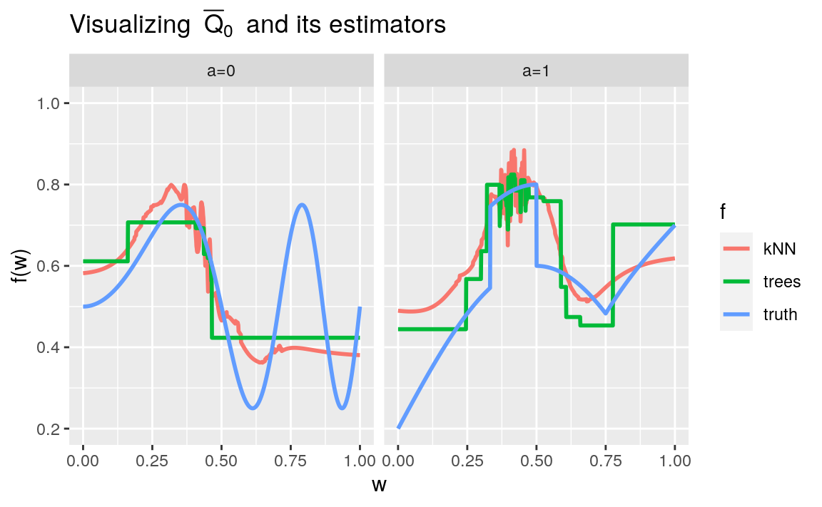
Figure 7.3: Comparing to their target two (machine learning-based) estimators of \(\Qbar_{0}\), one based on the \(k\)-nearest neighbors and the other on boosted trees.
7.7 ⚙ ☡ Qbar, machine learning-based algorithms
Using
estimate_Q, make your own machine learning-based algorithm for the estimation of \(\Qbar_{0}\).Train your algorithm on the same data set as \(\Algo_{\Qbar,\text{kNN}}\) and \(\Algo_{\Qbar,\text{trees}}\). If, like \(\Algo_{\Qbar,\text{trees}}\), your algorithm includes a fine-tuning procedure, comment upon the optimal, data-driven specification.
Plot your estimators of \(\Qbar_{0}(1,\cdot)\) and \(\Qbar_{0}(0,\cdot)\) on Figure 7.3.
7.8 Meta-learning/super learning
Without a great deal of previous experience or scientific expertise, it would have likely been difficult for us to a priori postulate which of the two above machine learning algorithms (or indeed the algorithm based on a working model) would perform better for estimation of \(\bar{Q}_0\). Rather than committing to one single algorithm, we may instead wish to resort to meta-learning or super learning. In this approach, one specifies a library of candidate algorithms for estimating a given nuisance parameter. Cross-validation is used to determine an ensemble (e.g. convex combination) of the algorithms that yields the best fit to the underlying function. In this way, one can learn in real time which algorithms tend to fit the data best and shift attention towards those algorithms.
In fact, if one knows nothing about the feature, then it is certain that it does not belong to whichever small finite-dimensional working model we may come up with.↩︎
See also the companion function
compute_lGbar_hat_AW(run?compute_lGbar_hat_AWto see its man page.↩︎Specifically, argument
kmax(maximum number of neighbors considered) is set to 5, argumentdistance(parameter of the Minkowski distance) is set to 2, and argumentkernelis set togaussian. The best value of \(k\) is chosen between 1 andkmaxby leave-one-out. No outer cross-validation is needed.↩︎Specifically, argument
mstop(number of boosting iterations for prediction) is one among 10, 20 and 30; argumentnu(stepsize of the shrinkage parameter) is one among 0.1 and 0.2; argumentmaxdepth(maximum depth of the base learner, a tree) is one among 1, 2 and 5. An outer 10-fold cross-validation is carried out to select the best combination of fine-tune parameters.↩︎