Section 10 Targeted minimum loss-based estimation
10.1 Motivations
10.1.1 Falling outside the parameter space
Section 9 introduced the one-step corrected estimator \(\psinos\) of \(\psi_0\). It is obtained by adding a correction term to an initial plug-in estimator \(\Psi(\Phat_{n})\), resulting in an estimator that is asymptotically linear with influence curve \(\IC = D^{*}(P_{0})\) under mild conditions (see Section 9.2 and the detailed proof there in Appendix C.2).
Unfortunately, the one-step estimator lacks a desirable feature of a plug-in estimator: plug-in estimators always lie in the parameter space whereas a one-step estimator does not necessarily do so. For example, it must also be true that \(\psi_0 = \Psi(P_{0}) \in [-1,1]\) yet it may be the case that \(\psinos \not\in[-1,1]\).
It is typically easy to shape an algorithm \(\Algo_{\Qbar}\) for the estimation of \(\Qbar_0\) to output estimators \(\Qbar_n\) that, like \(\Qbar_{0}\), take their values in \([0,1]\). The plug-in estimator \(\psi_{n}\) (8.1) based on such a \(\Qbar_{n}\) necessarily satisfies \(\psi_{n} \in [-1,1]\). However, the one-step estimator derived from \(\psi_{n}\) may fall outside of the interval if the correction term \(P_{n} D^{*} (\Phat_{n})\) is large.
10.1.2 The influence curve equation
Upon closer examination of the influence curve \(D^*(\Phat_{n})\), we see that this may occur more frequently when \(\ell \Gbar_n(A_i,W_i)\) is close to zero for at least some \(1 \leq i\leq n\). In words, this may happen if there are observations in our data set that we observed under actions \(A_i\) that were estimated to be unlikely given their respective contexts \(W_i\). In such cases, \(D^*(\Phat_n)(O_i)\), and consequently the one-step correction term, may be large and cause the one-step estimate to fall outside \([-1,1]\).
Another way to understand this behavior is to recognize the one-step estimator as an initial plug-in estimator that is corrected in the parameter space of \(\psi_0\). One of the pillars of targeted learning is to perform, instead, a correction in the parameter space of \(\Qbar_0\).
In particular, consider a law \(P_{n}^{*}\) estimating \(P_{0}\) that is compatible with the estimators \(\Qbar_n^*\), \(\Gbar_n\), and \(Q_{n,W}\), but moreover is such that \[\begin{equation} P_n D^*(P_{n}^*) = 0 \tag{10.1} \end{equation}\] or, at the very least, \[\begin{equation} P_n D^*(P_{n}^*) = o_{P_0}(1/\sqrt{n}). \tag{10.2} \end{equation}\] Achieving (10.1) is called solving the efficient influence curve equation. Likewise, achieving (10.2) is called approximately solving the influence curve equation.
If such estimators can be generated indeed, then the plug-in estimator \[\begin{equation*} \psi_n^* \defq \Psi(P_{n}^{*}) = \int \left(\Qbar_n^*(1,w) - \Qbar_n^*(0,w)\right) dQ_{n,W}(w) \end{equation*}\] is asymptotically linear with influence curve \(\IC = D^{*}(P_{0})\), under mild conditions. Moreover, by virtue of its plug-in construction, it has the additional property that in finite-samples \(\psi_n^*\) will always obey bounds on the parameter space.
10.1.3 A basic fact on the influence curve equation
Our strategy for constructing such a plug-in estimate begins by generating an initial estimator \(\Qbar_n\) of \(\Qbar_0\) based on an algorithm \(\Algo_{\Qbar}\) and an estimator \(\Gbar_n\) of \(\Gbar_0\) based on an algorithm \(\Algo_{\Gbar}\). These initial estimators should strive to be as close as possible to their respective targets. We use the empirical distribution \(Q_{n,W}\) as an estimator of \(Q_{0,W}\).
Now, recall the definition of \(D_{1}^{*}\) (3.4) and note that for any estimator \(\Qbar_n^*\) of \(\Qbar_0\) and a law \(P_n^{*}\) that is compatible with \(\Qbar_n^*\) and \(Q_{n,W}\), \[\begin{equation*} P_{n} D_{1} (P_{n}^{*}) = 0. \end{equation*}\] The proof can be found there in Appendix C.4.1.
In words, this shows that so long as we use the empirical distribution \(Q_{n,W}\) to estimate \(Q_{0,W}\), by its very construction achieving (10.1) or (10.2) is equivalent to solving \[\begin{equation} P_n D_{2}^*(P_{n}^*) = 0 \tag{10.3} \end{equation}\] or \[\begin{equation} P_n D_{2}^*(P_{n}^*) = o_{P_0}(1/\sqrt{n}). \tag{10.4} \end{equation}\]
It thus remains to devise a strategy for ensuring that \(P_n D_2^*(P_n^*) = 0\) or \(o_{P_0}(1/\sqrt{n})\).
10.2 Targeted fluctuation
Our approach to satisfying (10.3)21 hinges on revising our initial estimator \(\Qbar_n\) of \(\Qbar_0\). We propose a method for building an estimator of \(\Qbar_0\) that is “near to” \(\Qbar_n\), but is such that for any law \(P_n^*\) that is compatible with this revised estimator, \(P_n D^*(P_n^*) = 0\).22 Because \(\Qbar_n\) is our best (initial) estimator of \(\Qbar_0\), the new estimator that we shall build should be at least as good an estimator of \(\Qbar_0\) as \(\Qbar_n\). So first, we must propose a way to move between regression functions, and then we must propose a way to move to a new regression function that fits the data at least as well as \(\Qbar_n\).
Instead of writing “propos[ing] a way to move between regression functions” we may also have written “proposing a way to fluctuate a regression function,” thus suggesting very opportunely that the notion of fluctuation as discussed in Section 3.3 may prove instrumental to achieve the former objective.
10.2.1 ☡ Fluctuating indirectly
Let us resume the discussion where we left it at the end of Section 3.3.1. It is easy to show that the fluctuation \(\{P_{h} : h \in H\}\) of \(P\) in direction of \(s\) in \(\calM\) induces a fluctuation \(\{\Qbar_{h} : h \in H\}\) of \(\Qbar = \left.Q_{h}\right|_{h=0}\) in the space \(\calQ \defq \{\Qbar : P \in \calM\}\) of regression functions induced by model \(\calM\). Specifically we show there in Appendix C.4.2 that, for every \(h \in H\), the conditional mean \(\Qbar_{h}(A,W)\) of \(Y\) given \((A,W)\) under \(P_{h}\) is given by \[\begin{equation*}\Qbar_{h}(A,W) \defq \frac{\Qbar(A,W) + h \Exp_{P}(Ys(O) | A,W)}{1 + h \Exp_{P}(s(O)|A,W)}.\end{equation*}\]
We note that if \(s(O)\) depends on \(O\) only through \((A,W)\) then, abusing notation and writing \(s(A,W)\) for \(s(O)\), \[\begin{align} \Qbar_{h}(A,W) &= \frac{\Qbar(A,W) + h \Exp_{P}(Ys(A,W) | A,W)}{1 + h \Exp_{P}(s(A,W)|A,W)}\notag\\&=\frac{\Qbar(A,W) + h s(A,W)\Qbar(A,W)}{1 + h s(A,W)}\notag\\&=\Qbar(A,W).\tag{10.5} \end{align}\] In words, \(\Qbar\) is not fluctuated at all, that is, the laws \(P_{h}\) that are elements of the fluctuation share the same conditional mean of \(Y\) given \((A,W)\).23
However we find it easier in the present context, notably from a computational perspective, to fluctuate \(\Qbar_{n}\) directly in \(\calQ\), as opposed to indirectly through a fluctuation defined in \(\calM\) of a law compatible with \(\Qbar_{n}\). The next section introduces such a direct fluctuation.
10.2.2 Fluctuating directly
Set arbitrarily \(\Qbar \in \calQ\). The (direct) fluctuation of \(\Qbar\) that we propose to consider depends on a user-supplied \(\Gbar\). For any \(\Gbar\) such that \(0 < \ell\Gbar(A,W) < 1\), \(P_{0}\)-almost surely, the \(\Gbar\)-specific fluctuation model for \(\Qbar\) is \[\begin{equation} \calQ(\Qbar,\Gbar)\defq \left\{(w,a) \mapsto \Qbar_{h}(a,w) \defq \expit\left(\logit\left(\Qbar(a,w)\right) + h \frac{2a - 1}{\ell \Gbar(a,w)} \right) : t \in \bbR\right\} \subset \calQ. \tag{10.6} \end{equation}\]
Fluctuation \(\calQ(\Qbar,\Gbar)\) is a one-dimensional parametric model (indexed by the real-valued parameter \(h\)) that goes through \(\Qbar\) (at \(h=0\)). For each \(h \in \bbR\), \(\Qbar_{h} \in \calQ\) is the conditional mean of \(Y\) given \((A,W)\) under infinitely many laws \(P \in \calM\).
The following chunk of code represents three elements of the fluctuations \(\calQ(\Qbar_{0}, \Gbar_{0})\) and \(\calQ(\Qbar_{n,\text{trees}}, \Gbar_{0})\), where \(\Qbar_{n,\text{trees}}\) is an estimator of \(\Qbar_{0}\) derived by the boosted trees algorithm (see Section 7.6.3).
Qbar_hminus <- fluctuate(Qbar, Gbar, h = -1)
Qbar_hplus <- fluctuate(Qbar, Gbar, h = +1)

Qbar_trees <- wrapper(Qbar_hat_trees, FALSE)
Qbar_trees_hminus <- fluctuate(Qbar_trees, Gbar, h = -1)
Qbar_trees_hplus <- fluctuate(Qbar_trees, Gbar, h = +1)

tibble(w = seq(0, 1, length.out = 1e3)) %>%
  mutate(truth_0_1 = Qbar(cbind(A = 1, W = w)),
         truth_0_0 = Qbar(cbind(A = 0, W = w)),
         trees_0_1 = Qbar_trees(cbind(A = 1, W = w)),
         trees_0_0 = Qbar_trees(cbind(A = 0, W = w)),
         truth_hminus_1 = Qbar_hminus(cbind(A = 1, W = w)),
         truth_hminus_0 = Qbar_hminus(cbind(A = 0, W = w)),
         trees_hminus_1 = Qbar_trees_hminus(cbind(A = 1, W = w)),
         trees_hminus_0 = Qbar_trees_hminus(cbind(A = 0, W = w)),
         truth_hplus_1 = Qbar_hplus(cbind(A = 1, W = w)),
         truth_hplus_0 = Qbar_hplus(cbind(A = 0, W = w)),
         trees_hplus_1 = Qbar_trees_hplus(cbind(A = 1, W = w)),
         trees_hplus_0 = Qbar_trees_hplus(cbind(A = 0, W = w))) %>%
  pivot_longer(-w, names_to = "f", values_to = "value") %>%
  extract(f, c("f", "h", "a"), "([^_]+)_([^_]+)_([01]+)") %>%
  mutate(f = ifelse(f == "truth", "Q_0", "Q_n"),
         h = factor(ifelse(h == "0", 0, ifelse(h == "hplus", 1, -1)))) %>%
  mutate(a = paste0("a=", a),
         fh = paste0("(", f, ",", h, ")")) %>%
  ggplot +
  geom_line(aes(x = w, y = value, color = h, linetype = f, group = fh),
            size = 1) +
  labs(y = bquote(paste(f[h](a,w))),
       title = bquote("Visualizing three elements of two fluctuations of"
                      ~ bar(Q)[0] ~ "and" ~ bar(Q)[n])) +
  ylim(NA, 1) +
  facet_wrap(~ a)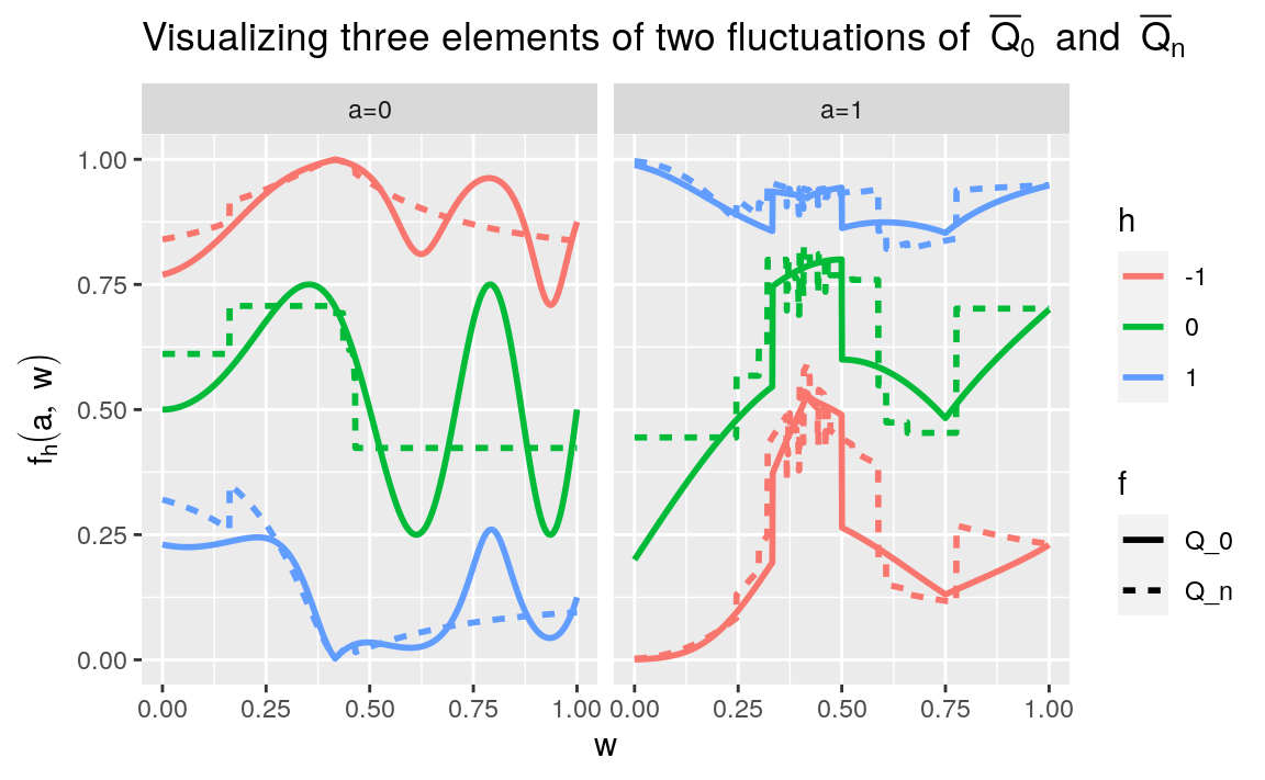
Figure 10.1: Representing three elements \(\Qbar_{h}\) of the fluctuations \(\calQ(\Qbar_{0}, \Gbar_{0})\) and \(\calQ(\Qbar_{n,\text{trees}}, \Gbar_{0})\), respectively, where \(\Qbar_{n,\text{trees}}\) is an estimator of \(\Qbar_{0}\) derived by the boosted trees algorithm (see Section 7.6.3). The three elements correspond to \(h=-1,0,1\). When \(h=0\), \(\Qbar_{h}\) equals either \(\Qbar_{0}\) or \(\Qbar_{n,\text{trees}}\), depending on which fluctuation is roamed.
10.2.3 ⚙ More on fluctuations
Justify the series of equalities in (10.5).
Justify that, in fact, if \(s(O)\) depends on \(O\) only through \((A,W)\) then the conditional law of \(Y\) given \((A,W)\) under \(P_{h}\) equals that under \(P\).
10.2.4 Targeted roaming of a fluctuation
Recall that our goal is to build an estimator of \(\Qbar_0\) that is at least as good as \(\Qbar_n\). We will look for this enhanced estimator in the fluctuation \(\calQ(\Qbar_{n}, \Gbar_{n})\) where \(\Gbar_{n}\) is an estimator of \(\Gbar_{0}\) that is bounded away from 0 and 1. Thus, the estimator writes as \(\Qbar_{n,h_{n}}\) for some data-driven \(h_{n} \in \bbR\). We will clarify why we do so at a later time
To assess the performance of all the candidates included in the fluctuation, we formally rely on the empirical risk function \(h \mapsto \Exp_{P_{n}} \left(L_{y} (\Qbar_{n,h})(O)\right)\) where \[\begin{equation*}\Exp_{P_{n}} \left(L_{y} (\Qbar_{n,h})(O)\right) = \frac{1}{n} \sum_{i=1}^{n} L_{y} (\Qbar_{n,h})(O_{i})\end{equation*}\] and the logistic (or negative binomial) loss function \(L_{y}\) is given by \[\begin{equation*} -L_{y}(f)(O) \defq Y \log f(A,W) + (1 - Y) \log \left(1 - f(A,W)\right) \tag{10.7} \end{equation*}\] for any function \(f:\{0,1\} \times [0,1] \to [0,1]\). This loss function is the counterpart of the loss function \(L_{a}\) defined in (7.1). The justification that we gave in Section 7.4.1 of the relevance of \(L_{a}\) also applies here, mutatis mutandis. In summary, the oracle risk \(\Exp_{P_{0}} \left(L_{y} (f)(O)\right)\) of \(f\) is a real-valued measure of discrepancy between \(\Qbar_{0}\) and \(f\); \(\Qbar_{0}\) minimizes \(f \mapsto \Exp_{P_{0}} \left(L_{y} (f)(O)\right)\) over the set of all (measurable) functions \(f:[0,1] \times \{0,1\} \times [0,1] \to [0,1]\); and a minimizer \(h_{0} \in \bbR\) of \(h \mapsto \Exp_{P_{0}} \left(L_{y} (\Qbar_{n,h})(O)\right)\) identifies the element of fluctuation \(\calQ(\Qbar_{n}, \Gbar_{n})\) that is closest to \(\Qbar_{0}\) (some details are given there in Appendix B.6).
It should not come as a surprise after this discussion that the aforementioned data-driven \(h_{n}\) is chosen to be the minimizer of the empirical risk function, i.e., \[\begin{equation*}h_{n} \defq \mathop{\arg\min}_{h \in \bbR} \Exp_{P_{n}} \left(L_{y} (\Qbar_{n,h})(O)\right).\end{equation*}\] The criterion is convex so the optimization program is well-posed.
The next chunk of code illustrates the search of an approximation of \(h_{n}\) over a grid of candidate values.
candidates <- seq(-0.01, 0.01, length.out = 1e4)
W <- obs[1:1e3, "W"]
A <- obs[1:1e3, "A"]
Y <- obs[1:1e3, "Y"]
lGAW <- compute_lGbar_hatAW(A, W, Gbar_hat)
QAW <- compute_Qbar_hatAW(A, W, Qbar_hat_trees)
risk <- sapply(candidates,
               function(h) {
                 QAW_h <- expit(logit(QAW)  + h * (2 * A - 1) / lGAW)
                 -mean(Y * log(QAW_h) + (1 - Y) * log(1 - QAW_h))
               })
idx_min <- which.min(risk)
idx_zero <- which.min(abs(candidates))[1]
labels <- c(expression(R[n](bar(Q)[list(n,hn)]^list(o))),
            expression(R[n](bar(Q)[list(n,0)]^list(o))))
risk %>% enframe %>%
  mutate(h = candidates) %>%
  filter(abs(h - h[idx_min]) <= abs(h[idx_min])) %>%
  ggplot() +
  geom_point(aes(x = h, y = value), color = "#CC6666") +
  geom_vline(xintercept = c(0, candidates[idx_min])) +
  geom_hline(yintercept = c(risk[idx_min], risk[idx_zero])) +
  scale_y_continuous(
    bquote("empirical logistic risk, " ~ R[n](bar(Q)[list(n,h)]^list(o))),
    trans = "exp", labels = NULL,
    sec.axis = sec_axis(~ .,
                        breaks = c(risk[idx_min], risk[idx_zero]),
                        labels = labels))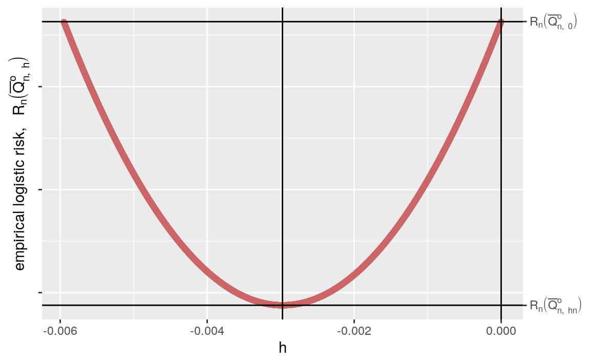
Figure 10.2: Representing the evolution of the empirical risk function as \(h\) ranges over a grid of values. One sees that the risk at \(h=0\) (i.e., the risk of \(\Qbar_{n}\)) is larger that the minimal risk, achieved at \(h \approx\) -0.003 (which must be close to that of the optimal \(\Qbar_{n,h_{n}}\)).
Figure 10.2 reveals how moving away slightly from \(h=0\) to the left (i.e., to \(h_{n}\) equal to -0.003, rounded to three decimal places) entails a decrease of the empirical risk. The gain is modest at the scale of the empirical risk, but considerable in terms of inference, as we explain below.
10.2.5 Justifying the form of the fluctutation
Let us define \(\Qbar_{n}^{*} \defq \Qbar_{n, h_{n}}\). We justify in two steps our assertion that moving from \(\left.\Qbar_{n}\right|_{h=0} = \Qbar_{n}\) to \(\Qbar_{n}^{*}\) along fluctuation \(\calQ(\Qbar_{n}, \Gbar_{n})\) has a considerable impact for the inference of \(\psi_{0}\).
First, we note that there is no need to iterate the updating procedure. Specifically, even if we tried to fluctuate \(\Qbar_{n}^{*}\) along the fluctuation \(\calQ(\Qbar_{n}^{*}, \Gbar_{n}) = \{\Qbar_{n,h'}^{*} : h' \in \bbR\}\) defined like \(\calQ(\Qbar_{n}, \Gbar_{n})\) (10.6) with \(\Qbar_{n,h_{n}}\) substituted for \(\Qbar_{n}\), then we would not move at all. This is obvious because there is a one-to-one smooth correspondence between the parameter \(h'\) indexing \(\calQ(\Qbar_{n}^{*}, \Gbar_{n})\) and the parameter \(h\) indexing \(\calQ(\Qbar_{n}, \Gbar_{n})\) (namely, \(h' = h + h_{n}\)). Therefore, the derivative of (the real-valued function over \(\bbR\)) \(h \mapsto \Exp_{P_n} \left(L_{y} (\Qbar_{n,h})(O)\right)\) evaluated at its minimizer \(h_{n}\) equals 0. Equivalently (see there in Appendix C.4.3 for a justification of the last but one equality below),
\[\begin{align}\notag \frac{d}{d h} & \left. \Exp_{P_{n}} \left(L_{y}(\Qbar_{n,h}^{*})(O)\right)\right|_{h=0} \\ \notag &= -\frac{1}{n}\left.\frac{d}{d h} \sum_{i=1}^{n} \left(Y_{i} \log \Qbar_{n,h}^{*}(A_{i}, W_{i}) + (1 - Y_{i}) \log\left(1 - \Qbar_{n,h}^{*}(A_{i}, W_{i})\right)\right)\right|_{h=0} \\ \notag &= -\frac{1}{n}\sum_{i=1}^{n} \left(\frac{Y_{i}}{\Qbar_{n}^{*}(A_{i}, W_{i})} - \frac{1 - Y_{i}}{1 - \Qbar_{n}^{*}(A_{i}, W_{i})}\right) \times \left.\frac{d}{d h} \Qbar_{n,h}^{*}(A_{i}, W_{i})\right|_{h=0} \\ \notag&= -\frac{1}{n}\sum_{i=1}^{n} \frac{Y_{i} - \Qbar_{n}^{*}(A_{i}, W_{i})}{\Qbar_{n}^{*}(A_{i}, W_{i}) \times \left(1 - \Qbar_{n}^{*}(A_{i}, W_{i})\right)} \left.\frac{d}{d h} \Qbar_{n,h}^{*}(A_{i}, W_{i})\right|_{h=0} \\ &= -\frac{1}{n}\sum_{i=1}^{n} \frac{2A_{i} - 1}{\ell\Gbar_{n}(A_{i}, W_{i})} \left(Y_{i} - \Qbar_{n}^{*}(A_{i}, W_{i})\right) = 0. \tag{10.8}\end{align}\]
Second, let \(P_{n}^{*}\) be a law in \(\calM\) such that the \(Q_{W}\), \(\Gbar\) and \(\Qbar\) features of \(P_{n}^{*}\) equal \(Q_{n,W}\), \(\Gbar_{n}\) and \(Q_{n}^{*}\), respectively. In other words, \(P_{n}^{*}\) is compatible with \(Q_{n,W}\), \(\Gbar_{n}\) and \(\Qbar_{n}^{*}\).24 Note that the last equality in (10.8) equivalently writes as \[\begin{equation*}P_{n} D_{2}^{*} (P_{n}^{*}) = 0.\end{equation*}\] Thus the (direct) fluctuation solves (10.3). Now, we have already argued in Section 10.1.3 that it also holds that \[\begin{equation*}P_{n} D_{1}^{*} (P_{n}^{*}) = 0.\end{equation*}\] Consequently, \(P_{n}^{*}\) solves the efficient influence curve equation, that is, satisfies (10.1). As argued in Section 10.1.2, it thus follows that the plug-in estimator \[\begin{equation*} \psi_n^* \defq \Psi(P_{n}^{*}) = \int \left(\Qbar_n^*(1,w) - \Qbar_n^*(0,w)\right) dQ_{n,W}(w) \end{equation*}\] is asymptotically linear with influence curve \(\IC = D^{*}(P_{0})\), under mild conditions. Moreover, by virtue of its plug-in construction, it has the additional property that in finite-samples \(\psi_n^*\) will always obey bounds on the parameter space.
10.2.6 ⚙ Alternative fluctuation
The following exercises will have you consider an alternative means of performing a fluctuation. For \(a = 0, 1\), consider the following fluctuation model for \(\Qbar^a \defq \Qbar(a,\cdot)\): \[\begin{equation} \calQ^a(\Qbar^a) \defq \left\{w \mapsto \Qbar_{h}^a(w) \defq \expit\left(\logit\left(\Qbar(a,w)\right) + h \right) : h \in \bbR\right\} \subset \calQ. \tag{10.9} \end{equation}\] Let \[\begin{equation*} \calQ^{\text{alt}}(\Qbar) \defq \left\{(a,w) \mapsto \Qbar_{h_0, h_1}(a,w) \defq a \times \Qbar_{h_{1}}^1(w) + (1-a) \Qbar_{h_{0}}^0(w) : h_{0}, h_{1} \in \bbR\right\} \end{equation*}\] be the fluctuation model for \(\Qbar\) that is implied by the two submodels for \(\Qbar^1\) and \(\Qbar^0\).
Also for a given \(\Gbar\) satisfying that \(0 < \ell\Gbar(A,W) < 1\), \(P_{0}\)-almost surely, and both \(a=0,1\), consider the loss function \(L_{y,\Gbar}^{a}\) given by \[\begin{equation*} L_{y,\Gbar}^{a} (f) (A,W) \defq\frac{\one\{A = a\}}{\ell\Gbar(A, W)} L_{y} (f)(O) \end{equation*}\] for any function \(f:\{0,1\} \times [0,1] \to [0,1]\), where \(L_{y}\) is defined in (10.7) above. It yields the empirical risk function \[\begin{equation*} (h_{0}, h_{1}) \mapsto \sum_{a = 0,1} \Exp_{P_{n}} \left(L^a_{y, \Gbar} (\Qbar^a_{n,h_a})(O)\right). \end{equation*}\]
Comment on the differences between these fluctuation model and loss function compared to those discussed above.
Visualize three elements of \(\calQ^{\text{alt}}(\Qbar_0)\) and \(\calQ^{\text{alt}}(\Qbar_n)\): choose three values for \((h_0, h_1)\) and reproduce Figure 10.1.
Argue that in order to minimize the empirical risk over all \((h_0, h_1) \in \bbR^2\), we may minimize over \(h_0 \in \bbR\) and \(h_1 \in \bbR\) separately.
Visualize how the empirical risk with \(\Gbar = \Gbar_n\) varies for different elements \(\Qbar_{n, h_0, h_1}\) of \(\calQ(\Qbar_n)\). For simplicity (and with the justification of problem 3), you may wish to make a separate figure (like Figure 10.2) for \(a = 0, 1\) that illustrates how the empirical risk varies as a function of \(h_a\) while setting \(h_{1 - a} = 0\).
☡ Justify the validity of \(L^a_{y, \Gbar}\) as a loss function for \(\Qbar^a_0\): show that amongst all functions that map \(w\) to \((0,1)\), the true risk \(\Exp_{P_0}\left(L^a_{y, \Gbar}(f)(O)\right)\) is minimized when \(f = \Qbar^a_0\).
☡ Argue that your answer to problem 2 also implies that the summed loss function \(\sum_{a=0,1} L^a_{y, \Gbar}\) is valid for \(\Qbar\).
☡ Justify the combination of these loss function and fluctuation by repeating the calculation in equation (10.8) above, mutatis mutandis.
10.3 Summary and perspectives
The procedure laid out in Section 10 is called targeted minimum loss-based estimation (TMLE). The nomenclature derives from its logistics. We first generated an (un-targeted) initial estimator of \(\Psi(P_0)\) by substituting for \(P_{0}\) a law \(\Phat_{n}\) compatible with initial estimators of some \(\Psi\)-specific relevant nuisance parameters. Then through loss-minimization, we built a targeted estimator by substituting for \(\Phat_{n}\) a law \(P_{n}^{*}\) compatible with the nuisance parameters that we updated in a targeted fashion.
The TMLE procedure was coined in 2006 by Mark van der Laan and Dan Rubin (Laan and Rubin 2006). It has since then been developed and applied in a great variety of contexts. We refer to the monographies (Laan and Rose 2011) and (Laan and Rose 2018) for a rich overview.
In summary, targeted learning bridges the gap between formal inference of finite-dimensional parameters \(\Psi(P_{0})\) of the law \(P_{0}\) of the data, via bootstrapping or influence curves, and data-adaptive, loss-based, machine learning estimation of \(\Psi\)-specific infinite-dimensional features thereof (the so-called nuisance parameters). A typical example concerns the super learning-based, targeted estimation of effect parameters defined as identifiable versions of causal quantities. The TMLE algorithm integrates completely the estimation of the relevant nuisance parameters by super learning (Laan, Polley, and Hubbard 2007). Under mild assumptions, the targeting step removes the bias of the initial estimators of the targeted effects. The resulting TMLEs enjoy many desirable statistical properties: among others, by being substitution estimators, they lie in the parameter space; they are often double-robust; they lend themselves to the construction of confidence regions.
The scientific community is always engaged in devising and promoting enhanced principles for sounder research through the better design of experimental and nonexperimental studies and the development of more reliable and honest statistical analyses. By focusing on prespecified analytic plans and algorithms that make realistic assumptions in more flexible nonparametric or semiparametric statistical models, targeted learning has been at the forefront of this concerted effort. Under this light, targeted learning notably consists in translating knowledge about the data and underlying data-generating mechanism into a realistic model; in expressing the research question under the form of a statistical estimation problem; in analyzing the statistical estimation problem within the frame of the model; in developing ad hoc algorithms grounded in theory and tailored to the question at stake to map knowledge and data into an answer coupled to an assessment of its trustworthiness.
Quoting (Laan and Rose 2018):
Over the last decade, targeted learning has been established as a reliable framework for constructing effect estimators and prediction functions. The continued development of targeted learning has led to new solutions for existing problems in many data structures in addition to discoveries in varied applied areas. This has included work in randomized controlled trials, parameters defined by a marginal structural model, case-control studies, collaborative TMLE, missing and censored data, longitudinal data, effect modification, comparative effectiveness research, aging, cancer, occupational exposures, plan payment risk adjustment, and HIV, as well as others. In many cases, these studies compared targeted learning techniques to standard approaches, demonstrating improved performance in simulations and realworld applications.
It is now time to resume our introduction to TMLE and to carry out an empirical investigation of its statistical properties in the context of the estimation of \(\psi_{0}\).
10.4 Empirical investigation
10.4.1 A first numerical application
Let us illustrate the principle of targeted minimum loss estimation by
updating the G-computation estimator built on the \(n=1000\) first observations
in obs by relying on \(\Algo_{\Qbar,\text{kNN}}\), that is, on the algorithm
for the estimation of \(\Qbar_{0}\) as it is implemented in estimate_Qbar with
its argument algorithm set to the built-in kknn_algo (see Section
7.6.2). In Section 9.3, we
performed a one-step correction of the same initial estimator.
The algorithm has been trained earlier on this data set and produced the
object Qbar_hat_kknn. The following chunk of code prints the initial
estimator psin_kknn, its one-step update psin_kknn_os, then applies the
targeting step and presents the resulting estimator:
(psin_kknn)
#> # A tibble: 1 × 2
#>   psi_n   sig_n
#>   <dbl>   <dbl>
#> 1 0.101 0.00306
(psin_kknn_os)
#> # A tibble: 1 × 3
#>    psi_n  sig_n    crit_n
#>    <dbl>  <dbl>     <dbl>
#> 1 0.0999 0.0171 -0.000633
(psin_kknn_tmle <- apply_targeting_step(head(obs, 1e3),
                                        wrapper(Gbar_hat, FALSE),
                                        wrapper(Qbar_hat_kknn, FALSE)))
#> # A tibble: 1 × 3
#>    psi_n  sig_n    crit_n
#>    <dbl>  <dbl>     <dbl>
#> 1 0.0999 0.0171 -2.05e-17
In the call to apply_targeting_step we provide (i) the data set at hand
(first line), (ii) the estimator Gbar_hat of \(\Gbar_{0}\) that we built
earlier by using algorithm \(\Algo_{\Gbar,1}\) (second line; see Section
7.4.2), (iii) the estimator Qbar_hat_kknn of \(\Qbar_{0}\)
(third line). Apparently, in this particular example, the one-step correction
and targeted correction updater similarly the initial estimator.
10.4.2 ⚙ A computational exploration
Consult the man page of function
apply_targeting_step(run?apply_targeting_step) and explain what is the role of its inputepsilon.Run the chunk of code below. What does it do? Hint: check out the chunks of code of Sections 7.6.2, 8.2.1 and 10.4.1.
epsilon <- seq(-1e-2, 1e-2, length.out = 1e2)
Gbar_hat_w <- wrapper(Gbar_hat, FALSE)
Qbar_kknn <- wrapper(Qbar_hat_kknn, FALSE)

psi_trees_epsilon <- sapply(epsilon, function(h) {
  apply_targeting_step(head(obs, 1e3), Gbar_hat_w,
                       Qbar_trees, epsilon = h) %>%
    select(psi_n, crit_n) %>% as.matrix
})
idx_trees <- which.min(abs(psi_trees_epsilon[2, ]))

psi_kknn_epsilon <- sapply(epsilon, function(h) {
  apply_targeting_step(head(obs, 1e3), Gbar_hat_w,
                       Qbar_kknn, epsilon = h) %>%
    select(psi_n, crit_n) %>% as.matrix
})
idx_kknn <- which.min(abs(psi_kknn_epsilon[2, ]))

rbind(t(psi_trees_epsilon), t(psi_kknn_epsilon)) %>% as_tibble %>%
  rename("psi_n" = V1, "crit_n" = V2) %>%
  mutate(type = rep(c("trees", "kknn"), each = length(epsilon))) %>%
  ggplot() +
  geom_point(aes(x = crit_n, y = psi_n, color = type)) +
  geom_vline(xintercept = 0) +
  geom_hline(yintercept = c(psi_trees_epsilon[1,idx_trees],
                            psi_kknn_epsilon[1,idx_kknn])) +
  labs(x = bquote(paste(P[n]~D^"*", (P[list(n,h)]^o))),
       y = bquote(Psi(P[list(n,h)]^o)))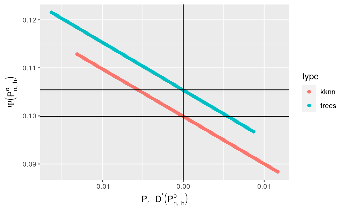
Figure 10.3: Figure produced when running the chunk of code from problem 2 in Section 10.4.2.
- Discuss the fact that the colored curves in Figure 10.3 look like segments.
10.4.3 Empirical investigation
To assess more broadly what is the impact of the targeting step, let us apply it to the estimators that we built in Section 8.4.3. In Section 9.3, we applied the one-step correction to the same estimators.
The object learned_features_fixed_sample_size already contains the estimated
features of \(P_{0}\) that are needed to perform the targeting step on the
estimators \(\psi_{n}^{d}\) and \(\psi_{n}^{e}\), thus we merely have to call the
function apply_targeting_step.
psi_tmle <- learned_features_fixed_sample_size %>%
  mutate(tmle_d =
           pmap(list(obs, Gbar_hat, Qbar_hat_d),
                ~ apply_targeting_step(as.matrix(..1),
                                 wrapper(..2, FALSE),
                                 wrapper(..3, FALSE))),
         tmle_e =
           pmap(list(obs, Gbar_hat, Qbar_hat_e),
                ~ apply_targeting_step(as.matrix(..1),
                                 wrapper(..2, FALSE),
                                 wrapper(..3, FALSE)))) %>%
  select(tmle_d, tmle_e) %>%
  pivot_longer(c(`tmle_d`, `tmle_e`),
               names_to = "type", values_to = "estimates") %>%
  extract(type, "type", "_([de])$") %>%
  mutate(type = paste0(type, "_targeted")) %>%
  unnest(estimates) %>%
  group_by(type) %>%
  mutate(sig_alt = sd(psi_n)) %>%
  mutate(clt_ = (psi_n - psi_zero) / sig_n,
         clt_alt = (psi_n - psi_zero) / sig_alt) %>%
  pivot_longer(c(`clt_`, `clt_alt`),
               names_to = "key", values_to = "clt") %>%
  extract(key, "key", "_(.*)$") %>%
  mutate(key = ifelse(key == "", TRUE, FALSE)) %>%
  rename("auto_renormalization" = key)

(bias_tmle <- psi_tmle %>%
   group_by(type, auto_renormalization) %>%
   summarize(bias = mean(clt)) %>% ungroup)
#> # A tibble: 4 × 3
#>   type       auto_renormalization     bias
#>   <chr>      <lgl>                   <dbl>
#> 1 d_targeted FALSE                -0.0147
#> 2 d_targeted TRUE                 -0.0313
#> 3 e_targeted FALSE                 0.0132
#> 4 e_targeted TRUE                 -0.00407

fig <- ggplot() +
  geom_line(aes(x = x, y = y),
            data = tibble(x = seq(-4, 4, length.out = 1e3),
                          y = dnorm(x)),
            linetype = 1, alpha = 0.5) +
  geom_density(aes(clt, fill = type, colour = type),
               psi_tmle, alpha = 0.1) +
  geom_vline(aes(xintercept = bias, colour = type),
             bias_tmle, size = 1.5, alpha = 0.5) +
  facet_wrap(~ auto_renormalization,
             labeller =
               as_labeller(c(`TRUE` = "auto-renormalization: TRUE",
                             `FALSE` = "auto-renormalization: FALSE")),
             scales = "free")

fig +
  labs(y = "",
       x = bquote(paste(sqrt(n/v[n]^{"*"})*
                        (psi[n]^{"*"} - psi[0]))))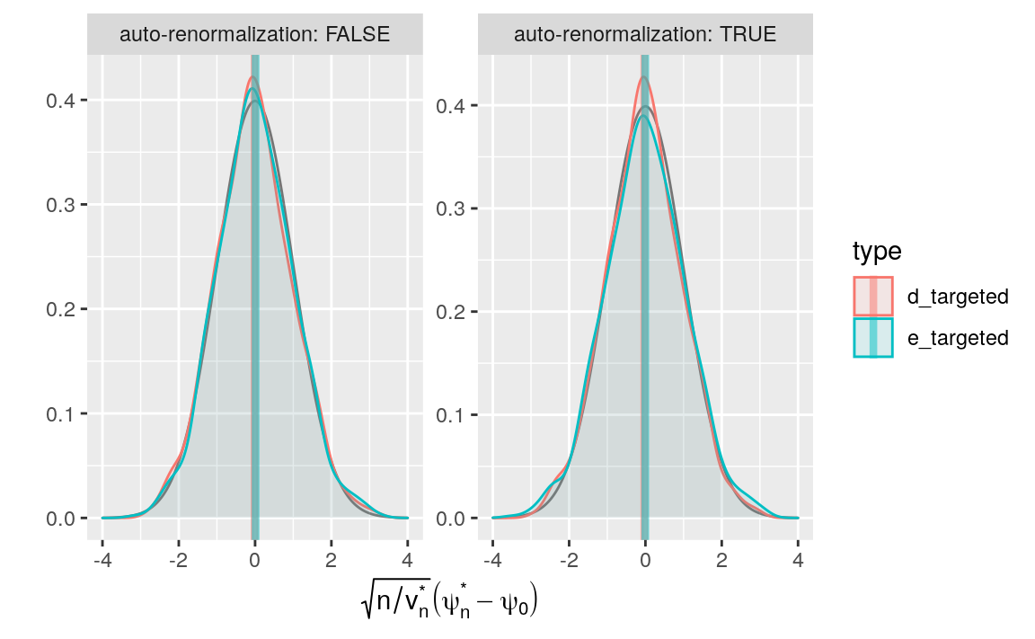
Figure 10.4: Kernel density estimators of the law of two targeted estimators of \(\psi_{0}\) (recentered with respect to \(\psi_{0}\), and renormalized). The estimators respectively hinge on algorithms \(\Algo_{\Qbar,1}\) (d) and \(\Algo_{\Qbar,\text{kNN}}\) (e) to estimate \(\Qbar_{0}\), and on a targeting step. Two renormalization schemes are considered, either based on an estimator of the asymptotic variance (left) or on the empirical variance computed across the 1000 independent replications of the estimators (right). We emphasize that the \(x\)-axis ranges differ between the left and right plots.
We see that the step of targeting is as promised: the bias of the resulting estimators is minimized relative to the naive estimators. Comparing these results to those obtain using one-step estimators (Section 9.3), we find quite similar performance between one-step and TMLE estimators.