Section 6 A simple inference strategy
6.1 A cautionary detour
Let us introduce first the following estimator:
\[\begin{align} \notag \psi_{n}^{a} &\defq \frac{\Exp_{P_{n}} (AY)}{\Exp_{P_{n}} (A)} - \frac{\Exp_{P_{n}} ((1-A)Y)}{\Exp_{P_{n}}(1-A)} \\ &= \frac{\sum_{i=1}^{n} \one\{A_{i}=Y_{i}=1\}}{\sum_{i=1}^{n} \one\{A_{i}=1\}} - \frac{\sum_{i=1}^{n} \one\{A_{i}=0,Y_{i}=1\}}{\sum_{i=1}^{n}\one\{A_{i}=0\}}. \tag{6.1} \end{align}\]
Note that \(\psi_n^a\) is simply the difference in sample means between observations with \(A = 1\) and observations with \(A = 0\). It estimates \[\begin{align*}\Phi(P_{0}) &\defq \frac{\Exp_{P_{0}} (AY)}{\Exp_{P_{0}} (A)} - \frac{\Exp_{P_{0}} ((1-A)Y)}{\Exp_{P_{0}} (1-A)}\\&= \Exp_{P_{0}} (Y | A=1) - \Exp_{P_{0}} (Y | A=0).\end{align*}\]
We seize this opportunity to demonstrate numerically that \(\psi_{n}^{a}\) does not estimate \(\Psi(P_{0})\) because, in general, \(\Psi(P_{0})\) and \(\Phi(P_{0})\) differ. This is apparent in the following alternative expression of \(\Phi(P_{0})\):
\[\begin{align*} \Phi(P_{0}) &= \Exp_{P_{0}} \left(\Exp_{P_0}(Y \mid A, W) |A=1) \right) - \Exp_{P_{0}} \left(\Exp_{P_0}(Y \mid A, W) | A=0\right)\\ &= \int \Qbar_{0}(1, w) dP_{0,W|A=1}(w) - \int \Qbar_{0}(0, w) dP_{0,W|A=0}(w). \end{align*}\]
Contrast the above equalities and (2.1). In the latter, the outer integral is against the marginal law of \(W\) under \(P_{0}\). In the former, the outer integrals are respectively against the conditional laws of \(W\) given \(A=1\) and \(A=0\) under \(P_{0}\). Thus \(\Psi(P_0)\) and \(\Phi(P_0)\) will enjoy equality when the conditional laws of \(W\) given \(A = 1\) and \(W\) given \(A = 0\) both equal the marginal law of \(W\). This can sometimes be ensured by design, as in an experiment where \(A\) is randomly allocated to observations, irrespective of \(W\). However, barring this level of experimental control, in general the naive estimator may lead us astray in our goal of drawing causal inference.
6.2 ⚙ Delta-method
Consider the next chunk of code:
compute_irrelevant_estimator <- function(obs) {
  obs <- as_tibble(obs)
  Y <- pull(obs, Y)
  A <- pull(obs, A)
  psi_n <- mean(A * Y) / mean(A) - mean((1 - A) * Y) / mean(1 - A)
  Var_n <- cov(cbind(A * Y, A, (1 - A) * Y, (1 - A)))
  phi_n <- c(1 / mean(A), -mean(A * Y) / mean(A)^2,
             -1 / mean(1 - A),
             mean((1 - A) * Y) / mean(1 - A)^2)
  var_n <- as.numeric(t(phi_n) %*% Var_n %*% phi_n)
  sig_n <- sqrt(var_n / nrow(obs))
  tibble(psi_n = psi_n, sig_n = sig_n)
}
Function compute_irrelevant_estimator computes the estimator \(\psi_{n}^{a}\)
(6.1) based on the data set in obs.
Introduce \(X_{n} \defq n^{-1}\sum_{i=1}^{n} \left(A_{i}Y_{i}, A_{i}, (1-A_{i})Y_{i}, 1-A_{i}\right)^{\top}\) and \(X \defq \left(AY, A, (1-A)Y, 1-A\right)^{\top}\). It happens that \(X_{n}\) is asymptotically Gaussian: as \(n\) goes to infinity,\[\begin{equation*}\sqrt{n} \left(X_{n} - \Exp_{P_{0}} (X)\right)\end{equation*}\] converges in law to the centered Gaussian law with covariance matrix \[\begin{equation*}V_{0} \defq \Exp_{P_{0}} \left((X - \Exp_{P_{0}} (X)) \times (X- \Exp_{P_{0}} (X))^{\top}\right).\end{equation*}\]
Let \(f:\bbR\times \bbR^{*} \times \bbR\times \bbR^{*}\) be given by \(f(r,s,t,u) = r/s - t/u\). The function is differentiable.
Check that \(\psi_{n}^{a} = f(X_{n})\). Point out the line where \(\psi_{n}^{a}\) is computed in the body of
compute_irrelevant_estimator. Also point out to the line where the above asymptotic variance of \(X_{n}\) is estimated with its empirical counterpart, say \(V_{n}\).☡ Argue how the delta-method yields that \(\sqrt{n}(\psi_{n}^{a} - \Phi(P_{0}))\) converges in law to the centered Gaussian law with a variance that can be estimated with \[\begin{equation} v_{n}^{a} \defq \nabla f(X_{n}) \times V_{n} \times \nabla f(X_{n})^{\top}. \tag{6.2} \end{equation}\]
Check that the gradient \(\nabla f\) of \(f\) is given by \(\nabla f(r,s,t,u) \defq (1/s, -r/s^{2}, -1/u, t/u^{2})\). Point out to the line where the asymptotic variance of \(\psi_{n}^{a}\) is estimated.
For instance,
(compute_irrelevant_estimator(head(obs, 1e3)))
#> # A tibble: 1 × 2
#>   psi_n  sig_n
#>   <dbl>  <dbl>
#> 1 0.126 0.0181
computes the numerical values of \(\psi_{n}^{a}\) and \(v_{n}^{a}\) based on the
1000 first observations in obs.
6.3 IPTW estimator assuming the mechanism of action known
6.3.1 A simple estimator
Let us assume for a moment that we know \(\Gbar_{0}\). This would have been the case indeed if we had experimental control over the actions taken by observational units, as in a randomized experiment. Note that, on the contrary, assuming \(\Qbar_{0}\) known would be difficult to justify.
Gbar <- get_feature(experiment, "Gbar")The alternative expression (2.7) suggests to estimate \(\Psi(P_{0})\) with
\[\begin{align} \psi_{n}^{b} &\defq \Exp_{P_{n}} \left( \frac{2A-1}{\ell \Gbar_{0}(A,W)} Y \right) \\ & = \frac{1}{n} \sum_{i=1}^{n} \left(\frac{2A_{i}-1}{ \ell\Gbar_{0}(A_{i},W_{i})}Y_{i} \right). \tag{6.3} \end{align}\]
Note how \(P_{n}\) is substituted for \(P_{0}\) in (6.3) relative to (2.7). However, we cannot call \(\psi_{n}^{b}\) a substitution estimator because it does not write as \(\Psi\) evaluated at an element of \(\calM\). This said, it is dubbed an IPTW (inverse probability of treatment weighted) estimator because of the denominators \(\ell\Gbar_{0}(A_{i},W_{i})\) in its definition.10
In Section 8.2, we develop another IPTW estimator that does not assume that \(\Gbar_{0}\) is known beforehand.
6.3.2 Elementary statistical properties
It is easy to check that \(\psi_{n}^{b}\) estimates \(\Psi(P_{0})\) consistently, but this is too little to request from an estimator of \(\psi_{0}\). Better, \(\psi_{n}^{b}\) also satisfies a central limit theorem: \(\sqrt{n} (\psi_{n}^{b} - \psi_{0})\) converges in law to a centered Gaussian law with asymptotic variance \[\begin{equation*}v^{b} \defq \Var_{P_{0}} \left(\frac{2A-1}{\ell\Gbar_{0}(A,W)}Y\right),\end{equation*}\] where \(v^{b}\) can be consistently estimated by its empirical counterpart
\[\begin{align} \tag{6.4} v_{n}^{b} &\defq \Var_{P_{n}} \left(\frac{2A-1}{\ell\Gbar_{0}(A,W)}Y\right) \\ &= \frac{1}{n} \sum_{i=1}^{n}\left(\frac{2A_{i}-1}{\ell\Gbar_{0} (A_{i},W_{i})} Y_{i} - \psi_{n}^{b}\right)^{2}. \end{align}\]
We investigate empirically the statistical behavior of \(\psi_{n}^{b}\) in Section 6.3.3.
6.3.3 Empirical investigation
The package tlrider includes compute_iptw, a function that implements the
IPTW inference strategy (simply run ?compute_iptw to see its man page). For
instance,
(compute_iptw(head(obs, 1e3), Gbar))
#> # A tibble: 1 × 2
#>   psi_n  sig_n
#>   <dbl>  <dbl>
#> 1 0.167 0.0533
computes the numerical values of \(\psi_{n}^{b}\) and \(v_{n}^{b}\) based
upon the 1000 first observations contained in obs.
The next chunk of code investigates the empirical behaviors of estimators
\(\psi_{n}^{a}\) and \(\psi_{n}^{b}\). As explained in Section 5,
we first make 1000 data sets out of the obs data set (second line), then
build the estimators on each of them (fourth and fifth lines). After the first
series of commands the object psi_hat_ab, a tibble, contains 2000
rows and four columns. For each smaller data set (identified by its id),
two rows contain the values of either \(\psi_{n}^{a}\) and
\(\sqrt{v_{n}^{a}}/\sqrt{n}\) (if type equals a) or \(\psi_{n}^{b}\) and
\(\sqrt{v_{n}^{b}}/\sqrt{n}\) (if type equals b).
After the second series of commands, the object psi_hat_ab contains, in
addition, the values of the recentered (with respect to \(\psi_{0}\)) and
renormalized \(\sqrt{n}/\sqrt{v_{n}^{a}} (\psi_{n}^{a} - \psi_{0})\) and
\(\sqrt{n}/\sqrt{v_{n}^{b}} (\psi_{n}^{b} - \psi_{0})\), where \(v_{n}^{a}\)
(6.2) and \(v_{n}^{b}\) (6.4) estimate the asymptotic
variances of \(\psi_{n}^{a}\) and \(\psi_{n}^{b}\), respectively. Finally,
bias_ab reports amounts of bias (at the renormalized scale).
We will refer to the recentering (always with respect to \(\psi_{0}\)) then renormalizing procedure as a renormalization scheme, because what may vary between two such procedures is the renormalization factor. We will judge whether or not the renormalization scheme is adequate for instance by comparing kernel density estimators of the law of estimators gone through a renormalization procedure with the standard normal density, as in Figure 6.1 below.
psi_hat_ab <- obs %>% as_tibble  %>%
  mutate(id = (seq_len(n()) - 1) %% iter) %>%
  nest(obs = c(W, A, Y)) %>%
  mutate(est_a = map(obs, ~ compute_irrelevant_estimator(.)),
         est_b = map(obs, ~ compute_iptw(as.matrix(.), Gbar))) %>%
  pivot_longer(c(`est_a`, `est_b`),
               names_to = "type", values_to = "estimates") %>%
  extract(type, "type", "_([ab])$") %>%
  unnest(estimates) %>% select(-obs)

(psi_hat_ab)
#> # A tibble: 2,000 × 4
#>      id type   psi_n  sig_n
#>   <dbl> <chr>  <dbl>  <dbl>
#> 1     0 a     0.140  0.0174
#> 2     0 b     0.0772 0.0546
#> 3     1 a     0.107  0.0169
#> 4     1 b     0.138  0.0541
#> 5     2 a     0.107  0.0172
#> 6     2 b     0.0744 0.0553
#> # … with 1,994 more rows

psi_hat_ab <- psi_hat_ab %>%
  group_by(id) %>%
  mutate(clt = (psi_n - psi_zero) / sig_n)

(psi_hat_ab)
#> # A tibble: 2,000 × 5
#> # Groups:   id [1,000]
#>      id type   psi_n  sig_n    clt
#>   <dbl> <chr>  <dbl>  <dbl>  <dbl>
#> 1     0 a     0.140  0.0174  3.23
#> 2     0 b     0.0772 0.0546 -0.109
#> 3     1 a     0.107  0.0169  1.40
#> 4     1 b     0.138  0.0541  1.01
#> 5     2 a     0.107  0.0172  1.38
#> 6     2 b     0.0744 0.0553 -0.159
#> # … with 1,994 more rows

(bias_ab <- psi_hat_ab %>%
   group_by(type) %>% summarize(bias = mean(clt), .groups = "drop"))
#> # A tibble: 2 × 2
#>   type    bias
#>   <chr>  <dbl>
#> 1 a     1.39
#> 2 b     0.0241

fig_bias_ab <- ggplot() +
  geom_line(aes(x = x, y = y),
            data = tibble(x = seq(-3, 3, length.out = 1e3),
                          y = dnorm(x)),
            linetype = 1, alpha = 0.5) +
  geom_density(aes(clt, fill = type, colour = type),
               psi_hat_ab, alpha = 0.1) +
  geom_vline(aes(xintercept = bias, colour = type),
             bias_ab, size = 1.5, alpha = 0.5)

fig_bias_ab +
  labs(y = "",
       x = bquote(paste(sqrt(n/v[n]^{list(a, b)})*
                        (psi[n]^{list(a, b)} - psi[0]))))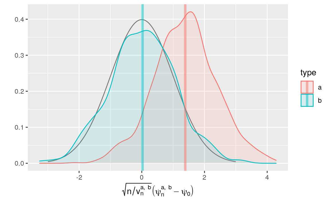
Figure 6.1: Kernel density estimators of the law of two estimators of \(\psi_{0}\) (recentered with respect to \(\psi_{0}\), and renormalized), one of them misconceived (a), the other assuming that \(\Gbar_{0}\) is known (b). Built based on 1000 independent realizations of each estimator.
By the above chunk of code, the averages of \(\sqrt{n/v_{n}^{a}} (\psi_{n}^{a} - \psi_{0})\) and \(\sqrt{n/v_{n}^{b}} (\psi_{n}^{b} - \psi_{0})\)
computed across the realizations of the two estimators are respectively equal
to 1.387 and
0.024 (see bias_ab). Interpreted as amounts of bias, those two
quantities are represented by vertical lines in Figure
6.1. The red and blue bell-shaped curves represent the
empirical laws of \(\psi_{n}^{a}\) and \(\psi_{n}^{b}\) (recentered with respect
to \(\psi_{0}\), and renormalized) as estimated by kernel density estimation.
The latter is close to the black curve, which represents the standard normal
density.
We could have used the alternative expression IPAW, where A (like action) is substituted for T (like treatment).↩︎