Section 3 Smoothness
3.1 Fluctuating smoothly
Within our view of the target parameter as a statistical mapping evaluated at the law of the experiment, it is natural to inquire of properties this functional enjoys. For example, we may be interested in asking how the value of \(\Psi(P)\) changes as we consider laws that get nearer to \(P\) in \(\calM\). If small deviations from \(P_0\) result in large changes in \(\Psi(P_0)\), then we might hypothesize that it will be difficult to produce stable estimators of \(\psi_0\). Fortunately, this turns out not to be the case for the mapping \(\Psi\), and so we say that \(\Psi\) is a smooth statistical mapping.
To discuss how \(\Psi(P)\) changes for distributions that get nearer to \(P\) in the model, we require a more concrete notion of what it means to get near to a distribution in a model. The notion hinges on fluctuations (or fluctuating models).
3.1.1 The another_experiment fluctuation
In Section 2.3.3, we discussed the nature of the
object called another_experiment that was created when we ran
example(tlrider):
another_experiment
#> A law for (W,A,Y) in [0,1] x {0,1} x [0,1].
#>
#> If the law is fully characterized, you can use method
#> 'sample_from' to sample from it.
#>
#> If you built the law, or if you are an _oracle_, you can also
#> use methods 'reveal' to reveal its relevant features (QW, Gbar,
#> Qbar, qY -- see '?reveal'), and 'alter' to change some of them.
#>
#> If all its relevant features are characterized, you can use
#> methods 'evaluate_psi' to obtain the value of 'Psi' at this law
#> (see '?evaluate_psi') and 'evaluate_eic' to obtain the efficient
#> influence curve of 'Psi' at this law (see '?evaluate_eic').
The message is a little misleading. Indeed, another_experiment is not a
law but, rather, a collection of laws indexed by a real-valued parameter
h. This oracular statement (we built the object!) is evident when one looks
again at the sample_from feature of another_experiment:
reveal(another_experiment)$sample_from
#> function(n, h) {
#>         ## preliminary
#>         n <- R.utils::Arguments$getInteger(n, c(1, Inf))
#>         h <- R.utils::Arguments$getNumeric(h)
#>         ## ## 'Gbar' and 'Qbar' factors
#>         Gbar <- another_experiment$.Gbar
#>         Qbar <- another_experiment$.Qbar
#>         ## sampling
#>         ## ## context
#>         params <- formals(another_experiment$.QW)
#>         W <- stats::runif(n, min = eval(params$min),
#>                    max = eval(params$max))
#>         ## ## action undertaken
#>         A <- stats::rbinom(n, size = 1, prob = Gbar(W))
#>         ## ## reward
#>         params <- formals(another_experiment$.qY)
#>         shape1 <- eval(params$shape1)
#>         QAW <- Qbar(cbind(A = A, W = W), h = h)
#>         Y <- stats::rbeta(n,
#>                           shape1 = shape1,
#>                           shape2 = shape1 * (1 - QAW) / QAW)
#>         ## ## observation
#>         obs <- cbind(W = W, A = A, Y = Y)
#>         return(obs)
#>       }
#> <bytecode: 0x56115cf79c38>
#> <environment: 0x56115878c6d8>
Let us call \(\Pi_{h} \in \calM\) the law encoded by another_experiment for a
given h taken in \(]-1,1[\). Note that \[\begin{equation*}\calP \defq
\{\Pi_h : h \in ]-1,1[\}\end{equation*}\] defines a collection of laws, i.e.,
a statistical model.
We say that \(\calP\) is a submodel of \(\calM\) because \(\calP \subset \calM\). Moreover, we say that this submodel is through \(\Pi_0\) since \(\Pi_{h} = \Pi_{0}\) when \(h = 0\). We also say that \(\calP\) is a fluctuation of \(\Pi_{0}\).
One could enumerate many possible submodels in \(\calM\) through \(\Pi_0\). It turns out that all that matters for our purposes is the form of the submodel in a neighborhood of \(\Pi_0\). We informally say that this local behavior describes the direction of a submodel through \(\Pi_0\). We formalize this notion Section 3.3.
We now have a notion of how to move through the model space \(P \in \calM\) and can study how the value of the parameter changes as we move away from a law \(P\). Above, we said that \(\Psi\) is a smooth parameter if it does not change “abruptly” as we move towards \(P\) in any particular direction. That is, we should hope that \(\Psi\) is differentiable along our submodel at \(P\). This idea too is formalized in Section 3.3. We now turn to illustrating this idea numerically.
3.1.2 Numerical illustration
The code below evaluates how the parameter changes for laws in \(\calP\), and
approximates the derivative of the parameter along the submodel \(\calP\) at
\(\Pi_0\). Recall that the numerical value of \(\Psi(\Pi_{0})\) has already been
computed and is stored in object psi_Pi_zero.
approx <- seq(-1, 1, length.out = 1e2)
psi_Pi_h <- sapply(approx, function(t) {
  evaluate_psi(another_experiment, h = t)
})
slope_approx <- (psi_Pi_h - psi_Pi_zero) / approx
slope_approx <- slope_approx[min(which(approx > 0))]
ggplot() +
  geom_point(data = data.frame(x = approx, y = psi_Pi_h), aes(x, y),
             color = "#CC6666") +
  geom_segment(aes(x = -1, y = psi_Pi_zero - slope_approx,
                   xend = 1, yend = psi_Pi_zero + slope_approx),
               arrow = arrow(length = unit(0.03, "npc")),
               color = "#9999CC") +
  geom_vline(xintercept = 0, color = "#66CC99") +
  geom_hline(yintercept = psi_Pi_zero, color = "#66CC99") +
labs(x = "h", y = expression(Psi(Pi[h]))) 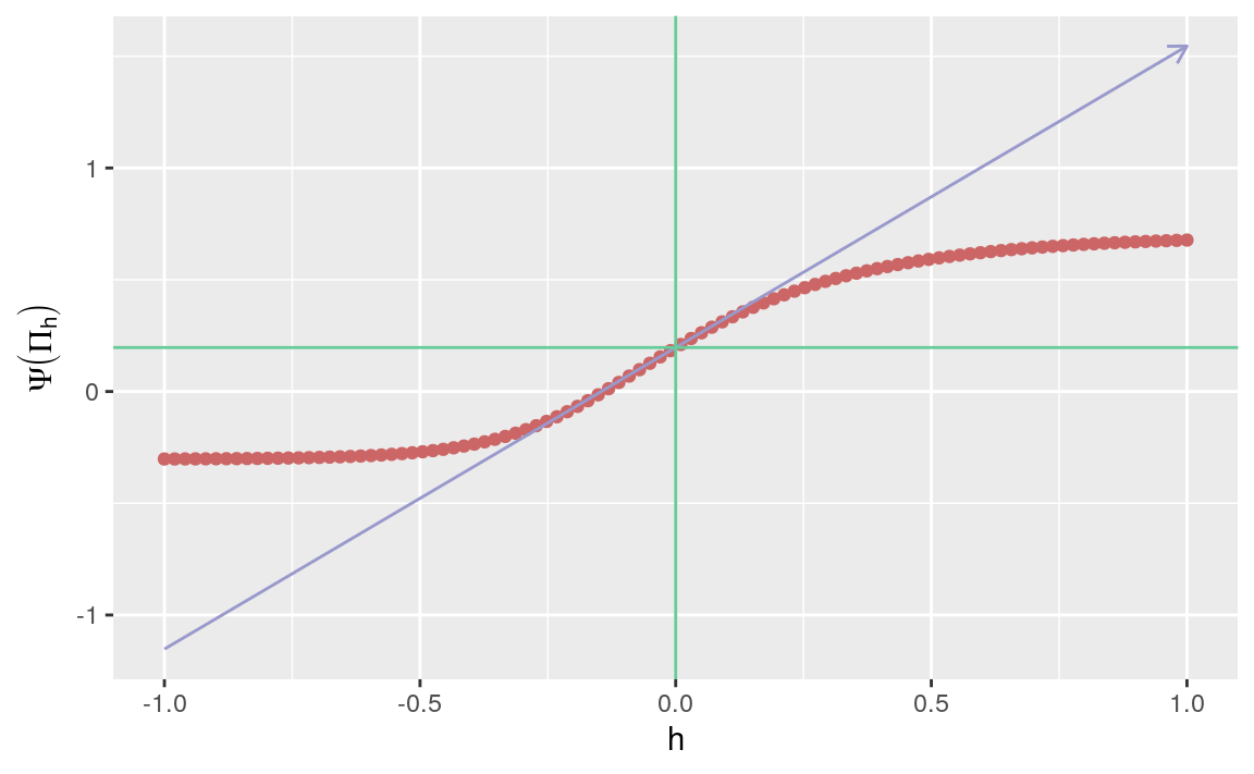
Figure 3.1: Evolution of statistical mapping \(\Psi\) along fluctuation \(\{\Pi_{h} : h \in H\}\).
The red curve represents the function \(h \mapsto \Psi(\Pi_{h})\). The blue line represents the tangent to the previous curve at \(h=0\), which indeed appears to be differentiable around \(h=0\). In Section 3.4, we derive a closed-form expression for the slope of the blue curve.
3.2 ⚙ Yet another experiment
Adapt the code from Problem 1 in Section 1.3 to visualize \(w \mapsto \Exp_{\Pi_h}(Y | A = 1, W = w)\), \(w \mapsto \Exp_{\Pi_h}(Y | A = 0, W=w)\), and \(w \mapsto \Exp_{\Pi_h}(Y | A = 1, W=w) - \Exp_{\Pi_h}(Y | A = 0, W=w)\), for \(h \in \{-1/2, 0, 1/2\}\).
Run the following chunk of code.
yet_another_experiment <- copy(another_experiment)
alter(yet_another_experiment,
      Qbar = function(AW, h){
        A <- AW[, "A"]
        W <- AW[, "W"]
        expit( logit( A * W + (1 - A) * W^2 ) +
               h * (2*A - 1) / ifelse(A == 1,
                                      sin((1 + W) * pi / 6),
                                      1 - sin((1 + W) * pi / 6)) *
               (Y - A * W + (1 - A) * W^2))
      })
Justify that
yet_another_fluctuationcharacterizes another fluctuation of \(\Pi_{0}\). Comment upon the similarities and differences between \(\{\Pi_{h} : h \in ]-1,1[\}\) and \(\{\Pi_{h}' : h \in ]-1,1[\}\).Repeat Problem 1 above with \(\Pi_{h}'\) substituted for \(\Pi_{h}\).
Re-produce Figure 3.1 for the \(\{\Pi_h' : h \in ]-1,1[\}\) fluctuation. Comment on the similarities and differences between the resulting figure and Figure 3.1. In particular, how does the behavior of the target parameter around \(h = 0\) compare between laws \(\Pi_0\) and \(\Pi_0'\)?
3.3 ☡ More on fluctuations and smoothness
3.3.1 Fluctuations
Let us now formally define what it means for statistical mapping \(\Psi\) to be smooth at every \(P \in \calM\). Let \(H\) be the interval \(]-1/M,M[\). For every \(h \in H\), we can define a law \(P_{h} \in \calM\) by setting \(P_{h} \ll P\)5 and \[\begin{equation} \frac{dP_h}{dP} \defq 1 + h s, \tag{3.1} \end{equation}\] where \(s : \calO\to \bbR\) is a (measurable) function of \(O\) such that \(s(O)\) is not equal to zero \(P\)-almost surely, \(\Exp_{P} (s(O)) = 0\), and \(s\) bounded by \(M\). We make the observation that \[\begin{equation} (i) \quad P_h|_{h=0} = P,\quad (ii) \quad \left.\frac{d}{dh} \log \frac{dP_h}{dP}(O)\right|_{h=0} =s(O). \tag{3.2} \end{equation}\]
Because of (i), \(\{P_{h} : h \in H\}\) is a submodel through \(P\), also referred to as a fluctuation of \(P\). The fluctuation is a one-dimensional submodel of \(\calM\) with univariate parameter \(h \in H\). We note that (ii) indicates that the score of this submodel at \(h = 0\) is \(s\). Thus, we say that the fluctuation is in the direction of \(s\).
Fluctuations of \(P\) do not necessarily take the same form as in (3.1). No matter how the fluctuation is built, for our purposes the most important feature of the fluctuation is its direction.
3.3.2 Smoothness and gradients
We are now prepared to provide a formal definition of smoothness of statistical mappings. We say that a statistical mapping \(\Psi\) is smooth at every \(P \in \calM\) if for each \(P \in \calM\), there exists a (measurable) function \(D^{*}(P) : \calO \to \bbR\) such that \(\Exp_{P}(D^{*}(P)(O)) = 0\), \(\Var_{P}(D^{*}(P)(O)) < \infty\), and, for every fluctuation \(\{P_{h} : h \in H\}\) with score \(s\) at \(h = 0\), the real-valued mapping \(h \mapsto \Psi(P_{h})\) is differentiable at \(h=0\), with a derivative equal to \[\begin{equation} \Exp_{P} \left( D^{*}(P)(O) s(O) \right). \tag{3.3} \end{equation}\] The object \(D^*(P)\) in (3.3) is called a gradient of \(\Psi\) at \(P\).6
3.3.3 A Euclidean perspective
This terminology has a direct parallel to directional derivatives in the calculus of Euclidean geometry. Recall that if \(f\) is a differentiable mapping from \(\bbR^p\) to \(\bbR\), then the directional derivative of \(f\) at a point \(x\) (an element of \(\bbR^p\)) in direction \(u\) (a unit vector in \(\bbR^p\)) is the scalar product of the gradient of \(f\) and \(u\). In words, the directional derivative of \(f\) at \(x\) can be represented as a scalar product of the direction that we approach \(x\) and the change of the function’s value at \(x\).
In the present problem, the law \(P\) is the point at which we evaluate the function \(\Psi\), the score \(s\) of the fluctuation is the direction in which we approach the point, and the gradient describes the change in the function’s value at the point.
3.3.4 The canonical gradient
In general, it is possible for many gradients to exist7. Yet, in the special case that the model is nonparametric, only a single gradient exists. The unique gradient is then referred to as the canonical gradient or, for reasons that will be clarified in Section 3.5, the efficient influence curve. In the more general setting, the canonical gradient may be defined as the minimizer of \(D\mapsto \Var_{P} (D(O))\) over the set of all gradients of \(\Psi\) at \(P\).
It is not difficult to check that the efficient influence curve of statistical mapping \(\Psi\) (2.6) at \(P \in \calM\) can be written as \[\begin{align} D^{*}(P) & \defq D_{1}^{*} (P) + D_{2}^{*} (P), \quad \text{where} \tag{3.4}\\ D_{1}^{*}(P) (O) &\defq \Qbar(1,W) - \Qbar(0,W) - \Psi(P), \notag\\ D_{2}^{*}(P) (O) &\defq \frac{2A-1}{\ell\Gbar(A,W)}(Y - \Qbar(A,W)).\notag \end{align}\]
A method from package tlrider evaluates the efficient influence curve at a
law described by an object of class LAW. It is called evaluate_eic. For
instance, the next chunk of code evaluates the efficient influence curve
\(D^{*}(P_{0})\) of \(\Psi\) (2.6) at \(P_{0} \in \calM\) that is
characterized by experiment:
eic_experiment <- evaluate_eic(experiment)The efficient influence curve \(D^{*}(P_{0})\) is a function from \(\calO\) to \(\bbR\). As such, it can be evaluated at the five independent observations drawn from \(P_{0}\) in Section 1.2.2. This is what the next chunk of code does:
(eic_experiment(five_obs))
#> [1] -0.0241 -0.0283  0.1829  0.0374 -0.0463
Finally, the efficient influence curve can be visualized as two images that represent \((w,y) \mapsto D^{*}(P_{0})(w,a,y)\) for \(a = 0,1\), respectively:
crossing(w = seq(0, 1, length.out = 2e2),
     a = c(0, 1),
     y = seq(0, 1, length.out = 2e2)) %>%
  mutate(eic = eic_experiment(cbind(Y=y,A=a,W=w))) %>%
  ggplot(aes(x = w, y = y, fill = eic)) +
  geom_raster(interpolate = TRUE) +
  geom_contour(aes(z = eic), color = "white") +
  facet_wrap(~ a, nrow = 1,
             labeller = as_labeller(c(`0` = "a = 0", `1` = "a = 1"))) +
  labs(fill = expression(paste(D^"*", (P[0])(w,a,y))))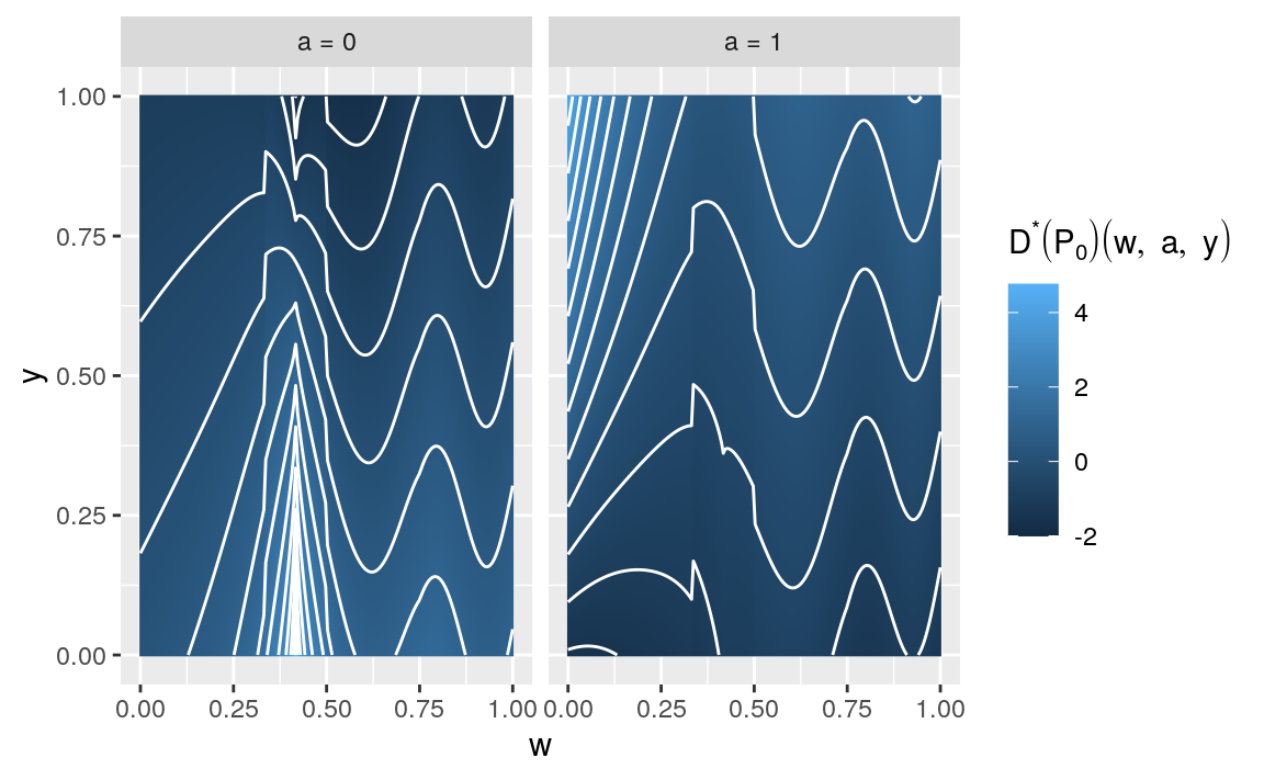
Figure 3.2: Visualizing the efficient influence curve \(D^{*}(P_{0})\) of \(\Psi\) (2.6) at \(P_{0}\), the law described by experiment.
3.4 A fresh look at another_experiment
We can give a fresh look at Section 3.1.2 now.
3.4.1 Deriving the efficient influence curve
It is not difficult (though cumbersome) to verify that, up to a constant, \(\{\Pi_{h} : h \in [-1,1]\}\) is a fluctuation of \(\Pi_{0}\) in the direction (in the sense of (3.1)) of
\[\begin{align} \notag\sigma_{0}(O) \defq &- 10 \sqrt{W} A \times \beta_{0} (A,W)\\ &\times\left(\log(1 - Y) + \sum_{k=0}^{3} \left(k + \beta_{0} (A,W)\right)^{-1}\right) + \text{constant}, \quad \text{where}\\ \beta_{0}(A,W)\defq & \frac{1 -\Qbar_{\Pi_{0}}(A,W)}{\Qbar_{\Pi_{0}}(A,W)}. \tag{3.5}\end{align}\]
Consequently, the slope of line in Figure 3.1 is equal to
\[\begin{equation} \Exp_{\Pi_{0}} (D^{*}(\Pi_{0}) (O) \sigma_{0}(O)). \tag{3.6} \end{equation}\]
Since \(D^{*}(\Pi_{0})\) is centered under \(\Pi_{0}\), knowing \(\sigma_{0}\) up to a constant is not problematic.
3.4.2 Numerical validation
In the following code, we check the above fact numerically. When we ran
example(tlrider), we created a function sigma0. The function implements
\(\sigma_{0}\) defined in (3.5):
sigma0
#> function(obs, law = another_experiment) {
#>   ## preliminary
#>   Qbar <- get_feature(law, "Qbar", h = 0)
#>   QAW <- Qbar(obs[, c("A", "W")])
#>   params <- formals(get_feature(law, "qY", h = 0))
#>   shape1 <- eval(params$shape1)
#>   ## computations
#>   betaAW <- shape1 * (1 - QAW) / QAW
#>   out <- log(1 - obs[, "Y"])
#>   for (int in 1:shape1) {
#>     out <- out + 1/(int - 1 + betaAW)
#>   }
#>   out <- - out * shape1 * (1 - QAW) / QAW *
#>            10 * sqrt(obs[, "W"]) * obs[, "A"]
#>   ## no need to center given how we will use it
#>   return(out)
#>  }
The next chunk of code approximates (3.6) pointwise and with a confidence interval of asymptotic level 95%:
eic_another_experiment <- evaluate_eic(another_experiment, h = 0)
obs_another_experiment <- sample_from(another_experiment, B, h = 0)
vars <- eic_another_experiment(obs_another_experiment) *
  sigma0(obs_another_experiment)

sd_hat <- sd(vars)
(slope_hat <- mean(vars))
#> [1] 1.35
(slope_CI <- slope_hat + c(-1, 1) *
   qnorm(1 - alpha / 2) * sd_hat / sqrt(B))
#> [1] 1.35 1.36
Equal to 1.349 (rounded to three decimal places —
hereafter, all rounding will be to three decimal places as well), the first
numerical approximation slope_approx is not too off!
3.5 ☡ Asymptotic linearity and statistical efficiency
3.5.1 Asymptotic linearity
Suppose that \(O_{1}, \ldots, O_{n}\) are drawn independently from \(P\in \calM\). If an estimator \(\psi_n\) of \(\Psi(P)\) can be written as
\[\begin{equation} \psi_n = \Psi(P) + \frac{1}{n}\sum_{i=1}^n \IC(O_i) + o_{P}(1/\sqrt{n}) \tag{3.7} \end{equation}\]
for some function \(\IC : \calO \to \bbR\) such that \(\Exp_P(\IC(O)) = 0\) and \(\Var_{P}(\IC(O)) < \infty\), then we say that \(\psi_n\) is asymptotically linear with influence curve \(\IC\). Asymptotically linear estimators are weakly convergent. Specifically, if \(\psi_n\) is asymptotically linear with influence curve \(\IC\), then
\[\begin{equation} \sqrt{n} (\psi_n - \Psi(P)) = \frac{1}{\sqrt{n}} \sum_{i=1}^n \IC(O_i) + o_P(1) \tag{3.8} \end{equation}\]
and, by the central limit theorem (recall that \(O_{1}, \ldots, O_{n}\) are independent), \(\sqrt{n} (\psi_n - \Psi(P))\) converges in law to a centered Gaussian distribution with variance \(\Var_P(\IC(O))\).
3.5.2 Influence curves and gradients
As it happens, influence curves of regular8 estimators are intimately related to gradients. In fact, if \(\psi_n\) is a regular, asymptotically linear estimator of \(\Psi(P)\) with influence curve \(\IC\), then it must be true that \(\Psi\) is a smooth parameter at \(P\) and that \(\IC\) is a gradient of \(\Psi\) at \(P\).
3.5.3 Asymptotic efficiency
Now recall that, in Section 3.3.4, we defined the canonical gradient as the minimizer of \(D \mapsto \Var_{P}(D(O))\) over the set of all gradients. Therefore, if \(\psi_{n}\) is a regular, asymptotically linear estimator of \(\Psi(P)\) (built from \(n\) independent observations drawn from \(P\)), then the asymptotic variance of \(\sqrt{n} (\psi_{n} - \Psi(P))\) cannot be smaller than the variance of the canonical gradient of \(\Psi\) at \(P\), i.e.,
\[\begin{equation} \tag{3.9}\Var_{P}(D^{*}(P)(O)). \end{equation}\]
In other words, (3.9) is the lower bound on the asymptotic variance of any regular, asymptotically linear estimator of \(\Psi(P)\). This bound is referred to as the Cramér-Rao bound. Any regular estimator that achieves this variance bound is said to be asymptotically efficient at \(P\). Because the canonical gradient is the influence curve of an asymptotically efficient estimator, it is often referred to as the efficient influence curve.
3.6 ⚙ Cramér-Rao bounds
- What does the following chunk do?
obs <- sample_from(experiment, B)
(cramer_rao_hat <- var(eic_experiment(obs)))
#> [1] 0.287- Same question about this one.
obs_another_experiment <- sample_from(another_experiment, B, h = 0)
(cramer_rao_Pi_zero_hat <-
   var(eic_another_experiment(obs_another_experiment)))
#> [1] 0.0946
With a large independent sample drawn from \(\Psi(P_0)\) (or \(\Psi(\Pi_0)\)), is it possible to construct a regular estimator \(\psi_{n}\) of \(\Psi(P_0)\) (or \(\Psi(\Pi_0)\)) such that the asymptotic variance of \(\sqrt{n}\) times \(\psi_{n}\) minus its target be smaller than the Cramér-Rao bound?
Is it easier to estimate \(\Psi(P_{0})\) or \(\Psi(\Pi_{0})\) (from independent observations drawn from either law)? In what sense? (Hint: you may want to compute a ratio.)
That is, \(P_{h}\) is dominated by \(P\): if an event \(A\) satisfies \(P(A) = 0\), then necessarily \(P_{h} (A) = 0\) too. Because \(P_{h} \ll P\), the law \(P_{h}\) has a density with respect to \(P\), meaning that there exists a (measurable) function \(f\) such that \(P_{h}(A) = \int_{o \in A} f(o) dP(o)\) for any event \(A\). The function is often denoted \(dP_{h}/dP\).↩︎
Interestingly, if a fluctuation \(\{P_{h} : h \in H\}\) satisfies (3.2) for a direction \(s\) such that \(s\neq 0\), \(\Exp_{P}(s(O)) = 0\) and \(\Var_{P} (s(O)) < \infty\), then \(h \mapsto \Psi(P_{h})\) is still differentiable at \(h=0\) with a derivative equal to (3.3) beyond fluctuations of the form (3.1).↩︎
This may be at first surprising given the parallel drawn in Section 3.3.3 to Euclidean geometry. However, it is important to remember that the model dictates fluctuations of \(P\) that are valid submodels with respect to the full model. In turn, this determines the possible directions from which we may approach \(P\). Thus, depending on the direction, (3.3) may hold with different choices of \(D^*\).↩︎
We can view \(\psi_{n}\) as the by product of an algorithm \(\Psihat\) trained on independent observations \(O_{1}, \ldots, O_{n}\) drawn from \(P\). We say that the estimator is regular at \(P\) if, for any direction \(s\neq 0\) such that \(\Exp_{P} (s(O)) = 0\) and \(\Var_{P} (s(O)) < \infty\) and fluctuation \(\{P_{h} : h \in H\}\) satisfying (3.2), the estimator \(\psi_{n,1/\sqrt{n}}\) of \(\Psi(P_{1/\sqrt{n}})\) obtained by training \(\Psihat\) on independent observations \(O_{1}\), , \(O_{n}\) drawn from \(P_{1/\sqrt{n}}\) is such that \(\sqrt{n} (\psi_{n,1/\sqrt{n}} - \Psi(P_{1/\sqrt{n}}))\) converges in law to a limit that does not depend on \(s\).↩︎