Section 2 The parameter of interest
2.1 The parameter of interest
2.1.1 Definition
It happens that we especially care for a finite-dimensional feature of \(P_{0}\) that we denote by \(\psi_{0}\). Its definition involves two of the aforementioned infinite-dimensional features, the marginal law \(Q_{0,W}\) of \(W\) and the conditional mean \(\Qbar_{0}\) of \(Y\) given \(A\) and \(W\): \[\begin{align} \psi_{0} &\defq \int \left(\Qbar_{0}(1, w) - \Qbar_{0}(0, w)\right) dQ_{0,W}(w) \tag{2.1}\\ \notag &= \Exp_{P_{0}} \left(\Exp_{P_0}(Y \mid A = 1, W) - \Exp_{P_0}(Y \mid A = 0, W) \right). \end{align}\]
Acting as oracles, we can compute explicitly the numerical value of
\(\psi_{0}\). The evaluate_psi method makes it very easy (simply run
?estimate_psi to see the man page of the method):
(psi_zero <- evaluate_psi(experiment))
#> [1] 0.0832
2.1.2 A causal interpretation
Our interest in \(\psi_{0}\) is of causal nature. Taking a closer look at the
sample_from feature of experiment reveals indeed that the random making of
an observation \(O\) drawn from \(P_{0}\) can be summarized by the following
directed acyclic graph:
dagify(
  Y ~ A + Y1 + Y0, A ~ W, Y1 ~ W, Y0 ~ W,
  labels = c(Y = "Actual reward",
             A = "Action",
             Y1 = "Counterfactual reward\n of action 1",
             Y0 = "Counterfactual reward\n of action 0",
             W = "Context of action"),
  coords = list(
    x = c(W = 0, A = -1, Y1 = 1.5, Y0 = 0.25, Y = 1),
    y = c(W = 0, A = -1, Y1 = -0.5, Y0 = -0.5, Y = -1)),
  outcome = "Y",
  exposure = "A",
  latent = c("Y0", "Y1")) %>% tidy_dagitty %>%
  ggdag(text = TRUE, use_labels = "label") + theme_dag_grey()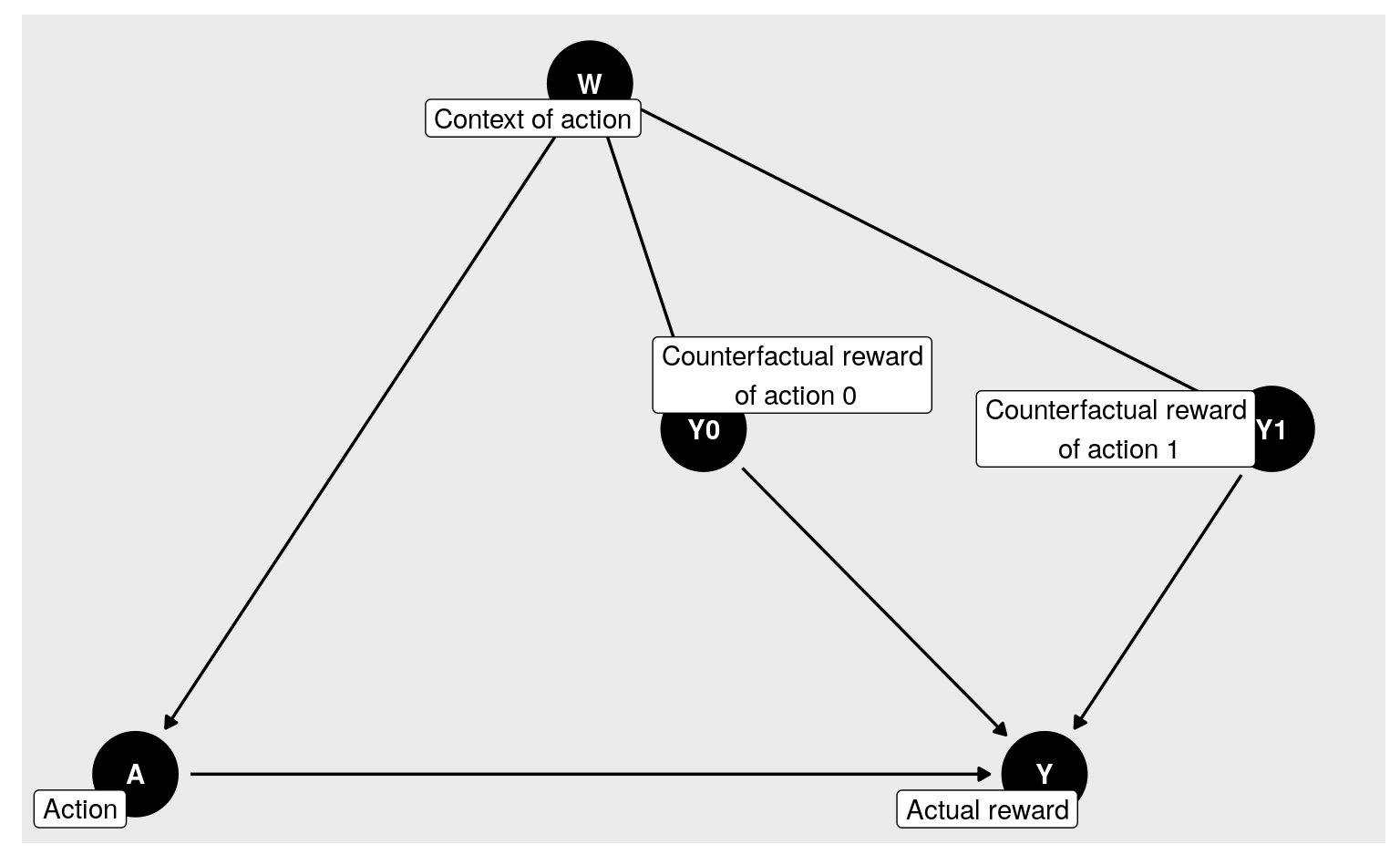
Figure 2.1: Directed acyclic graph summarizing the inner causal mechanism at play in experiment.
In words, the experiment unfolds like this (see also Section B.1):
a context of action \(W \in [0,1]\) is randomly generated;
two counterfactual rewards \(Y_{0}\in [0,1]\) and \(Y_{1}\in [0,1]\) are generated conditionally on \(W\);
an action \(A \in \{0,1\}\) (among two possible actions called \(a=0\) and \(a=1\)) is undertaken, (i) knowing the context but not the counterfactual rewards, and (ii) in such a way that both actions can always be considered;
the action yields a reward \(Y\), which equals either \(Y_{0}\) or \(Y_{1}\) depending on whether action \(a=0\) or \(a=1\) has been undertaken;
summarize the course of the experiment with \(O \defq (W, A, Y)\), thus concealing \(Y_{0}\) and \(Y_{1}\).
The above description of the experiment is useful to reinforce what it means
to run the “ideal” experiment by setting argument ideal to TRUE in a call
to sample_from for experiment (see Section 2.1.3).
Doing so triggers a modification of the nature of the experiment, enforcing
that the counterfactual rewards \(Y_{0}\) and \(Y_{1}\) be part of the summary of
the experiment eventually. In light of the above enumeration,
\[\begin{equation*} \bbO \defq (W, Y_{0}, Y_{1}, A, Y) \end{equation*}\] is
output, as opposed to its summary measure \(O\). This defines another
experiment and its law, that we denote \(\bbP_{0}\).
It is straightforward to show that
\[\begin{align} \psi_{0} &= \Exp_{\bbP_{0}} \left(Y_{1} - Y_{0}\right) \tag{2.2} \\ &= \Exp_{\bbP_{0}}(Y_1) - \Exp_{\bbP_{0}}(Y_0). \notag \end{align}\]
Thus, \(\psi_{0}\) describes the average difference of the two counterfactual rewards. In other words, \(\psi_{0}\) quantifies the difference in average of the reward one would get in a world where one would always enforce action \(a=1\) with the reward one would get in a world where one would always enforce action \(a=0\). This said, it is worth emphasizing that \(\psi_{0}\) is a well-defined parameter beyond its causal interpretation, and that it describes a standardized association between the action \(A\) and reward \(Y\).
2.1.3 A causal computation
We can use our position as oracles to sample observations from the ideal
experiment. We call sample_from for experiment with its argument ideal
set to TRUE in order to numerically approximate \(\psi_{0}\). By the law of
large numbers, the following code approximates \(\psi_{0}\) and shows it
approximate value.
B <- 1e6
ideal_obs <- sample_from(experiment, B, ideal = TRUE)
(psi_approx <- mean(ideal_obs[, "Yone"] - ideal_obs[, "Yzero"]))
#> [1] 0.0829
The object psi_approx contains an approximation to \(\psi_0\) based on B
observations from the ideal experiment. The random sampling of observations
results in uncertainty in the numerical approximation of \(\psi_0\). This
uncertainty can be quantified by constructing a 95% confidence interval for
\(\psi_0\). The central limit theorem and Slutsky’s lemma allow us to
build such an interval as follows.
sd_approx <- sd(ideal_obs[, "Yone"] - ideal_obs[, "Yzero"])
alpha <- 0.05
(psi_approx_CI <- psi_approx + c(-1, 1) *
   qnorm(1 - alpha / 2) * sd_approx / sqrt(B))
#> [1] 0.0823 0.0835
We note that the interpretation of this confidence interval is that in 95% of
draws of size B from the ideal data generating experiment, the true value of
\(\psi_0\) will be contained in the generated confidence interval.
2.2 ⚙ An alternative parameter of interest
Equality (2.2) shows that parameter \(\psi_0\) (2.1) is the difference in average rewards if we enforce action \(a = 1\) rather than \(a = 0\). An alternative way to describe the rewards under different actions involves quantiles as opposed to averages.
Let \[\begin{equation*} Q_{0,Y}(y, A, W) \defq \int_{0}^y q_{0,Y}(u, A, W) du \end{equation*}\] be the conditional cumulative distribution of reward \(Y\) given \(A\) and \(W\), evaluated at \(y \in ]0,1[\), that is implied by \(P_0\). For each action \(a \in \{0,1\}\) and \(c \in ]0,1[\), introduce
\[\begin{equation} \gamma_{0,a,c} \defq \inf \left\{y \in ]0,1[ : \int Q_{0,Y}(y, a, w) dQ_{0,W}(w) \ge c \right\}. \tag{2.3} \end{equation}\] (Note: \(\inf\) merely generalizes \(\min\), accounting for the fact that the minimum may fail to be achieved.)
It is not very difficult to check (see Problem 1 below) that \[\begin{equation}\gamma_{0,a,c} = \inf\left\{y \in ]0,1[ : \Pr_{\bbP_{0}}(Y_a \leq y) \geq c\right\}. \tag{2.4}\end{equation}\] Thus, \(\gamma_{0,a,c}\) can be interpreted as the \(c\)-th quantile reward when action \(a\) is enforced. The difference \[\begin{equation}\delta_{0,c} \defq \gamma_{0,1,c} - \gamma_{0,0,c} \tag{2.5}\end{equation}\] is the \(c\)-th quantile counterpart to parameter \(\psi_{0}\) (2.1).
☡ Prove (2.4).
☡ Compute the numerical value of \(\gamma_{0,a,c}\) for each \((a,c) \in \{0,1\} \times \{1/4, 1/2, 3/4\}\) using the appropriate features of
experiment(seerelevant_features). Based on these results, report the numerical value of \(\delta_{0,c}\) for each \(c \in \{1/4, 1/2, 3/4\}\).Approximate the numerical values of \(\gamma_{0,a,c}\) for each \((a,c) \in \{0,1\} \times \{1/4, 1/2, 3/4\}\) by drawing a large sample from the “ideal” data experiment and using empirical quantile estimates. Deduce from these results a numerical approximation to \(\delta_{0,c}\) for \(c \in \{1/4, 1/2, 3/4\}\). Confirm that your results closely match those obtained in the previous problem.
2.3 The statistical mapping of interest
The noble way to define a statistical parameter is to view it as the value of a statistical mapping at the law of the experiment of interest. Beyond the elegance, this has paramount statistical implications.
2.3.1 Opening discussion
Oftentimes, the premise of a statistical analysis is presented like this. One assumes that the law \(P_{0}\) of the experiment of interest belongs to a statistical model \[\begin{equation*}\{P_{\theta} : \theta \in T\}\end{equation*}\] (where \(T\) is some index set). The statistical model is identifiable, meaning that if two elements \(P_{\theta}\) and \(P_{\theta'}\) coincide, then necessarily \(\theta = \theta'\). Therefore, there exists a unique \(\theta_{0} \in T\) such that \(P_{0} = P_{\theta_{0}}\), and one wishes to estimate \(\theta_{0}\).
For instance, each \(P_{\theta}\) could be the Gaussian law with mean \(\theta \in T \defq \bbR\) and variance 1, and one could wish to estimate the mean \(\theta_{0}\) of \(P_{0}\). To do so, one could rely on \(n\) observations \(X_{1}\), , \(X_{n}\) drawn independently from \(P_{0}\). The empirical mean \[\begin{equation*}\theta_{n} \defq \frac{1}{n} \sum_{i=1}^{n} X_{i}\end{equation*}\] estimates \(\theta_{0}\). More generally, if we assume that \(\Var_{P_{0}} (X_{1})\) is finite, then \(\theta_{n}\) satisfies many useful properties. In particular, it can be used to construct confidence intervals.
Of course, the mean of a law is defined beyond the small model \(\{P_{\theta} : \theta \in \bbR\}\). Let \(\calM\) be the set of laws \(P\) on \(\bbR\) such that \(\Var_{P}(X)\) is finite. In particular, \(P_{0} \in \calM\). For every \(P \in \calM\), the mean \(\Exp_{P}(X)\) is well defined. Thus, we can introduce the statistical mapping \(\Theta : \calM \to \bbR\) given by \[\begin{equation*}\Theta(P) \defq \Exp_{P}(X).\end{equation*}\]
Interestingly, the empirical measure \(P_{n}\)3 is an element of \(\calM\). Therefore, the statistical mapping \(\Theta\) can be evaluated at \(P_{n}\): \[\begin{equation*}\Theta(P_{n}) = \frac{1}{n} \sum_{i=1}^{n} X_{i} = \theta_{n}.\end{equation*}\] We recover the empirical mean, and understand that it is a substitution estimator of the mean: in order to estimate \(\Theta(P_{0})\), we substitute \(P_{n}\) for \(P_{0}\) within \(\Theta\).4
Substitution-based estimators are particularly valuable notably because they, by construction, satisfy all the constraints to which the targeted parameter is subjected. For example, if \(X\) is a binary random variable and the support of all distributions in our model is \(\{0,1\}\), then \(\Theta\) can be interpreted as the probability that \(X = 1\), a quantity known to live in the interval \([0,1]\). A substitution estimator will also be guaranteed to fall into this interval. Some of the estimators that we will build together are substitution-based, some are not.
2.3.2 The parameter as the value of a statistical mapping at the experiment
We now go back to our main topic of interest. Suppose we know beforehand that \(O\) drawn from \(P_{0}\) takes its values in \(\calO \defq [0,1] \times \{0,1\} \times [0,1]\) and that \(\Gbar_{0}(W) \defq \Pr_{P_{0}}(A=1|W)\) is bounded away from zero and one \(Q_{0,W}\)-almost surely (this is the case indeed). Then we can define model \(\calM\) as the set of all laws \(P\) on \(\calO\) such that \[\begin{equation*}\Gbar(W) \defq \Pr_{P}(A=1|W)\end{equation*}\] is bounded away from zero and one \(Q_{W}\)-almost surely, where \(Q_{W}\) is the marginal law of \(W\) under \(P\).
Let us also define generically \(\Qbar\) as \[\begin{equation*}\Qbar (A,W) \defq \Exp_{P} (Y|A, W).\end{equation*}\] Note how we have suppressed the dependence of \(\Gbar\) and \(\Qbar\) on \(P\) for notational simplicity.
Central to our approach is viewing \(\psi_{0}\) as the value at \(P_{0}\) of the statistical mapping \(\Psi\) from \(\calM\) to \([0,1]\) characterized by \[\begin{align} \Psi(P) &\defq \int \left(\Qbar_P(1, w) - \Qbar_P(0, w)\right) dQ_{W}(w) \tag{2.6}\\ &= \Exp_{P} \left(\Qbar_P(1, W) - \Qbar_P(0, W)\right), \notag \end{align}\] a clear extension of (2.1) where, for once, we make the dependence of \(\Qbar\) on \(P\) explicit to emphasize how \(\Psi(P)\) truly depends on \(P\).
2.3.3 The value of the statistical mapping at another experiment
When we ran example(tlrider) earlier, we created an object called
another_experiment:
another_experiment
#> A law for (W,A,Y) in [0,1] x {0,1} x [0,1].
#>
#> If the law is fully characterized, you can use method
#> 'sample_from' to sample from it.
#>
#> If you built the law, or if you are an _oracle_, you can also
#> use methods 'reveal' to reveal its relevant features (QW, Gbar,
#> Qbar, qY -- see '?reveal'), and 'alter' to change some of them.
#>
#> If all its relevant features are characterized, you can use
#> methods 'evaluate_psi' to obtain the value of 'Psi' at this law
#> (see '?evaluate_psi') and 'evaluate_eic' to obtain the efficient
#> influence curve of 'Psi' at this law (see '?evaluate_eic').
reveal(another_experiment)
#> $QW
#> function(x, min = 1/10, max = 9/10){
#>              stats::dunif(x, min = min, max = max)
#>       }
#> <environment: 0x56115878c6d8>
#>
#> $Gbar
#> function(W) {
#>         sin((1 + W) * pi / 6)
#>       }
#> <environment: 0x56115878c6d8>
#>
#> $Qbar
#> function(AW, h) {
#>         A <- AW[, "A"]
#>         W <- AW[, "W"]
#>         expit( logit( A *  W + (1 - A) * W^2 ) +
#>                h * 10 * sqrt(W) * A )
#>       }
#> <environment: 0x56115878c6d8>
#>
#> $qY
#> function(obs, Qbar, shape1 = 4){
#>         AW <- obs[, c("A", "W")]
#>         QAW <- Qbar(AW)
#>         stats::gdbeta(Y,
#>                       shape1 = shape1,
#>                       shape2 = shape1 * (1 - QAW) / QAW)
#>       }
#> <environment: 0x56115878c6d8>
#>
#> $sample_from
#> function(n, h) {
#>         ## preliminary
#>         n <- R.utils::Arguments$getInteger(n, c(1, Inf))
#>         h <- R.utils::Arguments$getNumeric(h)
#>         ## ## 'Gbar' and 'Qbar' factors
#>         Gbar <- another_experiment$.Gbar
#>         Qbar <- another_experiment$.Qbar
#>         ## sampling
#>         ## ## context
#>         params <- formals(another_experiment$.QW)
#>         W <- stats::runif(n, min = eval(params$min),
#>                    max = eval(params$max))
#>         ## ## action undertaken
#>         A <- stats::rbinom(n, size = 1, prob = Gbar(W))
#>         ## ## reward
#>         params <- formals(another_experiment$.qY)
#>         shape1 <- eval(params$shape1)
#>         QAW <- Qbar(cbind(A = A, W = W), h = h)
#>         Y <- stats::rbeta(n,
#>                           shape1 = shape1,
#>                           shape2 = shape1 * (1 - QAW) / QAW)
#>         ## ## observation
#>         obs <- cbind(W = W, A = A, Y = Y)
#>         return(obs)
#>       }
#> <environment: 0x56115878c6d8>
(two_obs_another_experiment <- sample_from(another_experiment, 2, h = 0))
#>          W A     Y
#> [1,] 0.720 1 0.372
#> [2,] 0.616 1 0.670
By taking an oracular look at the output of reveal(another_experiment), we
discover that the law \(\Pi_{0} \in \calM\) encoded by default (i.e., with
h=0) in another_experiment differs starkly from \(P_{0}\).
However, the parameter \(\Psi(\Pi_{0})\) is well defined. Straightforward algebra shows that \(\Psi(\Pi_{0}) = 59/300\). The numeric computation below confirms the equality.
(psi_Pi_zero <- evaluate_psi(another_experiment, h = 0))
#> [1] 0.197
round(59/300, 3)
#> [1] 0.197
2.4 ⚙ Alternative statistical mapping
We now resume the exercise of Section 2.2. Like we did in Section 2.3, we introduce a generic version of the relevant features \(q_{0,Y}\) and \(Q_{0,Y}\). Specifically, we define \(q_{Y}(y,A,W)\) to be the conditional density of \(Y\) given \(A\) and \(W\), evaluated at \(y\), that is implied by a generic \(P \in \calM\). Similarly, we use \(Q_{Y}\) to denote the corresponding cumulative distribution function.
The covariate-adjusted \(c\)-th quantile reward for action \(a \in \{0,1\}\), \(\gamma_{0,a,c}\) (2.3), may be viewed as the value at \(P_{0}\) of a mapping \(\Gamma_{a,c}\) from \(\calM\) to \([0,1]\) characterized by \[\begin{equation*} \Gamma_{a,c}(P) = \inf\left\{y \in ]0,1[ : \int Q_{Y}(y,a,w) dQ_W(w) \ge c \right\}. \end{equation*}\] The difference in \(c\)-th quantile rewards, \(\delta_{0,c}\) (2.5), may similarly be viewed as the value at \(P_{0}\) of a mapping \(\Delta_c\) from \(\calM\) to \([0,1]\), characterized by \[\begin{equation*} \Delta_c(P) \defq \Gamma_{1,c}(P) - \Gamma_{0,c}(P). \end{equation*}\]
Compute the numerical value of \(\Gamma_{a,c}(\Pi_0)\) for \((a,c) \in \{0,1\} \times \{1/4, 1/2, 3/4\}\) using the relevant features of
another_experiment. Based on these results, report the numerical value of \(\Delta_c(\Pi_0)\) for each \(c \in \{1/4, 1/2, 3/4\}\).Approximate the value of \(\Gamma_{0,a,c}(\Pi_{0})\) for \((a,c) \in \{0,1\} \times \{1/4, 1/2, 3/4\}\) by drawing a large sample from the “ideal” data experiment and using empirical quantile estimates. Deduce from these results a numerical approximation to \(\Delta_{0,c} (\Pi_{0})\) for each \(c \in \{1/4, 1/2, 3/4\}\). Confirm that your results closely match those obtained in the previous problem.
Building upon the code you wrote to solve the previous problem, construct a confidence interval with asymptotic level \(95\%\) for \(\Delta_{0,c} (\Pi_{0})\), with \(c \in \{1/4, 1/2, 3/4\}\).
2.5 Representations
In Section 2.3, we reoriented our view of the target parameter to be that of a statistical functional of the law of the observed data. Specifically, we viewed the parameter as a function of specific features of the observed data law, namely \(Q_{W}\) and \(\Qbar\).
2.5.1 Yet another representation
It is straightforward to show an equivalent representation of the parameter as
\[\begin{align} \notag \psi_{0} &= \int \frac{2a - 1}{\ell\Gbar_0(a,w)} y dP_0(w,a,y) \\ \tag{2.7} &= \Exp_{P_0} \left( \frac{2A - 1}{\ell\Gbar_{0}(A,W)} Y \right). \end{align}\] Viewing again the parameter as a statistical mapping from \(\calM\) to \([0,1]\), it also holds that \[\begin{align} \notag \Psi(P) &= \int \frac{2a-1}{\ell\Gbar(a,w)} y dP(w,a,y) \\ \tag{2.8} &= \Exp_{P}\left(\frac{2A - 1}{\ell\Gbar_{0}(A,W)} Y \right). \end{align}\]
2.5.2 From representations to estimation strategies
Our reason for introducing this alternative view of the target parameter will become clear when we discuss estimation of the target parameter. Specifically, the representations (2.1) and (2.7) naturally suggest different estimation strategies for \(\psi_0\), as hinted in Section 2.3.1. The former suggests building an estimator of \(\psi_0\) using estimators of \(\Qbar_0\) and of \(Q_{W,0}\). The latter suggests building an estimator of \(\psi_0\) using estimators of \(\ell\Gbar_0\) and of \(P_0\).
We return to these ideas in later sections.
2.6 ⚙ Alternative representation
- ☡ Show that for \(a' = 0,1\), \(\gamma_{0,a',c}\) as defined in (2.3) can be equivalently expressed as \[\begin{equation*}\inf \left\{z \in ]0,1[ : \int \frac{\one\{a = a'\}}{\ell\Gbar(a',W)} \one\{y \le z\} dP_0(w,a,y) \ge c \right\}.\end{equation*}\]
The empirical measure \(P_{n}\) is the law such that (i) \(X\) drawn from \(P_{n}\) takes its values in \(\{X_{1}, \ldots, X_{n}\}\), and (ii) \(X=X_{i}\) with probability \(n^{-1}\)↩︎
There are many interesting parameters \(\Theta\) for which \(\Theta(P_n)\) is not defined, see for instance (2.6), our parameter of main interest.↩︎