mediation-test • mediation.test

In this vignette, we illustrate the use of the package mediation.test by reproducing the simulation study reported in Miles and Chambaz (2024). Our objective is to compare the finite sample performances of our proposed tests with those of the delta method, joint significance, and van Garderen and van Giersbergen (henceforth vGvG, Garderen and Giersbergen (2022)) tests.

library(mediation.test)
library(tibble)
library(ggplot2)
theme_set(theme_gray(base_size = 5))
set.seed(1)

1 Simulation settings

Simulation scenarios

We will sample independently $k=1e5$ data points from $t$ -distributions with $(n-1)$ degrees of freedom and noncentrality parameters $\sqrt{n}(\delta_x , \delta_y)$ , where $n=50$ . Three simulation scenarios are considered:

$\delta_x$ and $\delta_y$ vary jointly from 0 to 0.4;
$\delta_y=0.2$ is fixed while $\delta_x$ varies from 0 to 0.4;
$\delta_y=0$ is fixed while $\delta_x$ varies from 0 to 0.6, thereby exploring empirical type I error across a range of parameter values within the composite null hypothesis space.

To do so, we will repeatedly use the function defined below.

n_obs <- 50

simulate <- function(delta_x, delta_y, k = 1e5, n = n_obs) {
    Xn <- rt(k, n - 1, sqrt(n) * delta_x)
    Yn <- rt(k, n - 1, sqrt(n) * delta_y)
    Zn <- cbind(Xn, Yn)
    return(Zn)
}

All the testing procedures will aim for a type I error $\alpha = 0.05$ .

alpha <- 0.05

Minimax optimal test

Three version of the minimax optimal test will be evaluated using the function mediation_test_minimax:

the standard version, using the normal approximation of the test statistic;
the test based on the corresponding (conservative) $p$ -value defined in the Supplementary Materials of Miles and Chambaz (2024);
a truncated minimax optimal test at level $d = 0.1$ , in order to make a fair comparison with the vGvG test, whose rejection region is 0.1 away from the null hypothesis space.

sample_size <- Inf
quantile_function <- qnorm
truncation <- 0.1

Bayes risk optimal test

Three versions of the Bayes risk optimal test will be evaluated using the function mediation_test_Bayes:

the standard version with 0-1 loss function,
the standard version with quadratic loss function,
and the constrained test with quadratic loss function.

We rely on the “maps” of rejection probabilities embarked in the package. In both the constrained and truncated tests, we also use a truncation at level $d = 0.1$ . Each “map” associates a rejection probability to every square $\left[\frac{B(i-1-m)}{m}, \frac{B(i-m)}{m}\right ] \times \left[\frac{B(j-1-m)}{m}, \frac{B(j-m)}{m}\right]$ with $B = 2 \Phi^{-1}(1 - \alpha/2)$ , $m=64$ and $1 \leq i,j \leq 2m$ .

m <- 64
map_01 <- map_01_0.05
map_quad <- map_quad_0.05
map_quad_trunc <- map_quad_0.05_0.1

For instance, this is what map_quad looks like:

plot(map_quad)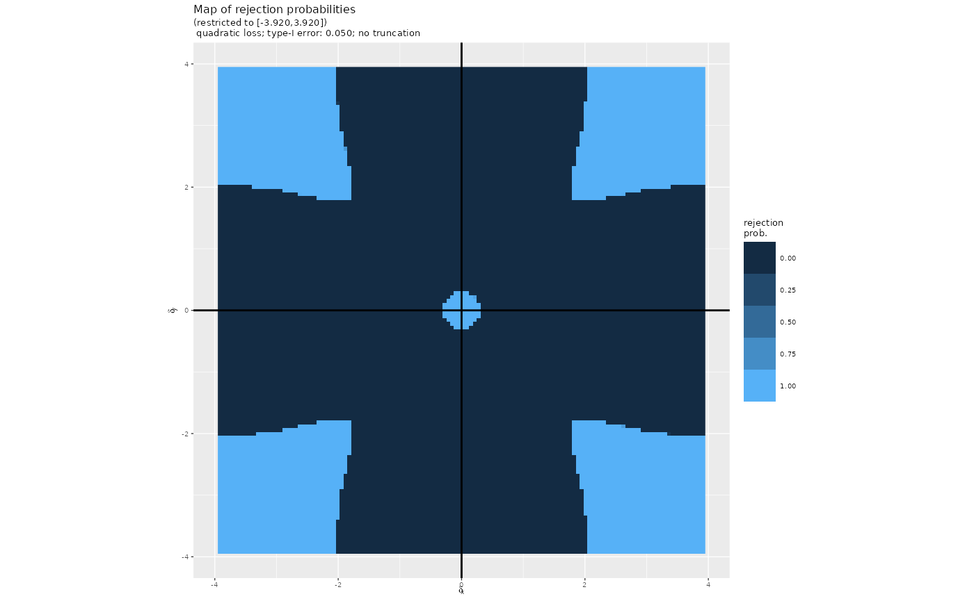

Had m been different (and alpha, truncation for that matter too), we would have relied on the function compute_map_rejection_probs to compute the corresponding maps.

if (!(alpha == 0.05 & m == 64 & truncation == 0.1)) {
    map_01 <- compute_map_rejection_probs(
        alpha = alpha,
        K = m,
        loss = "0-1",
        truncation = 0,
        return_solver = FALSE)
    map_quad <- compute_map_rejection_probs(
        alpha = alpha,
        K = m,
        loss = "quad",
        truncation = 0,
        return_solver = FALSE)
    map_quad_trunc <- compute_map_rejection_probs(
        alpha = alpha,
        K = m,
        loss = "quad",
        truncation = truncation,
        return_solver = FALSE)
}

Other testing procedures

Our minimax optimal and Bayes risk optimal tests will be compared to the delta method, joint significance, and vGvG tests.

delta_method_test <- function(Zn, alpha) {
    abs(Zn[, 1] * Zn[, 2]) / sqrt(apply(Zn^2, 1, sum)) >
        qnorm(1 - alpha / 2)
}
joint_significance_test <- function(Zn, alpha, quantile_function = qnorm) {
    abs(Zn[, 1]) > quantile_function(1 - alpha / 2) &
        abs(Zn[, 2]) > quantile_function(1 - alpha / 2)
}
vGvG_test <- function(Zn, alpha = 0.05) {
    if (alpha == 0.05) {
        g <- function(t) {
            tabs <- abs(t)
            x <- c(0., 0.1, 0.11, 0.13, 0.14, 0.15, 1.35, 1.36, 1.37,
                   1.44, 1.45, 2.05, 2.06, 2.07, 2.08, 2.09, 2.1)
            y <- c(0., 0.1, 0.106723, 0.106723, 0.106724, 0.106724,
                   1.30583, 1.31286, 1.3131, 1.3131, 1.3175, 1.9175,
                   1.9275, 1.9375, 1.9475, 1.9575, 1.95996)
            ifelse(tabs >= 2.1, 1.95996, approx(x, y, xout = tabs)$y)
        }
        out <- pmin(abs(Zn[, 1]), abs(Zn[, 2])) >
            g(pmax(abs(Zn[, 1]), abs(Zn[, 2])))
    } else {
        out <- rep(NA, nrow(Zn))
    }
    return(out)
}

2 Scenario (a)

We first initialize the vectors that will receive the empirical powers.

P <- 20
pow_nms <- c("pow_minimax",  "pow_minimax_trunc", "pow_minimax_pval",
             "pow_Bayes_01",  "pow_Bayes_quad",  "pow_Bayes_quad_constr", 
             "pow_delta", "pow_js", "pow_vGvG")
for (pow in pow_nms) {
    assign(pow, rep(0, P + 1), envir = .GlobalEnv)
}

We are now in a position to conduct the Monte Carlo analysis. To avoid unnecessary repetitions, we define a function called run_simulation that we will call repeatedly.

delta_x <- delta_y <- seq(0, .4, length.out = P + 1)

run_simulation <- function() {
    for (j in 1:(P + 1)) {
        ## ########## ##
        ## simulating ##
        ## ########## ##
        Zn <- simulate(delta_x[j], delta_y[j])
        ## ####### ##
        ## testing ##
        ## ####### ##
        R_minimax <- mediation_test_minimax(Zn,
                                            alpha = alpha,
                                            truncation = 0,
                                            sample_size = sample_size,
                                            compute_pvals = TRUE)
        R_minimax_pval <- R_minimax$pval <= alpha
        R_minimax_trunc <- mediation_test_minimax(Zn,
                                                  alpha = alpha,
                                                  truncation = truncation,
                                                  sample_size = sample_size,
                                                  compute_pvals = FALSE)
        R_Bayes_01 <- mediation_test_Bayes(Zn,
                                           map_01,
                                           truncation = 0)
        R_Bayes_quad <- mediation_test_Bayes(Zn,
                                             map_quad,
                                             truncation = 0)
        R_Bayes_quad_constr <- mediation_test_Bayes(Zn,
                                                    map_quad_trunc,
                                                    truncation = truncation)
        R_delta <- delta_method_test(Zn, alpha)
        R_js <- joint_significance_test(Zn, alpha, quantile_function)
        R_vGvG <- vGvG_test(Zn, alpha)
        ## ################ ##
        ## evaluating power ##
        ## ################ ##
        pow_minimax[j] <- mean(R_minimax$decision)
        pow_minimax_pval[j] <- mean(R_minimax_pval)
        pow_minimax_trunc[j] <- mean(R_minimax_trunc$decision)
        pow_Bayes_01[j] <- mean(R_Bayes_01$decision)
        pow_Bayes_quad[j] <- mean(R_Bayes_quad$decision)
        pow_Bayes_quad_constr[j] <- mean(R_Bayes_quad_constr$decision)
        pow_delta[j] <- mean(R_delta)
        pow_js[j] <- mean(R_js)
        pow_vGvG[j] <- mean(R_vGvG)
    }
    list(pow_minimax, pow_minimax_trunc, pow_Bayes_01, pow_Bayes_quad,
         pow_Bayes_quad_constr, pow_delta, pow_js, pow_minimax_pval, pow_vGvG)
}

## ###################### ##
## running the simulation ##
## ###################### ##
pow_a <- run_simulation()

## ####################### ##
## colllecting the results ##
## ####################### ##
pow_scenario_a <- tibble(delta = rep(delta_x, 9),
                         power = unlist(pow_a),
                         test = c(rep("MMO", P + 1),
                                  rep("MMO trunc", P + 1),
                                  rep("BRO 0-1", P + 1),
                                  rep("BRO quad", P + 1),
                                  rep("BRO q-cnst", P + 1),
                                  rep("Delta", P + 1),
                                  rep("JS", P + 1),
                                  rep("MMO pval", P + 1),
                                  rep("vGvG", P + 1)))

fig_scenario_a <- ggplot(data = pow_scenario_a) + 
    geom_line(aes(
        x = delta, y = power, group = test,
        color = test,
        ),
        linewidth = 0.5) + 
    geom_vline(xintercept = 0) + 
    geom_hline(yintercept = 0) + 
    geom_hline(yintercept = alpha, linetype = "dashed") +
    xlab(expression(delta[x]))
(fig_scenario_a)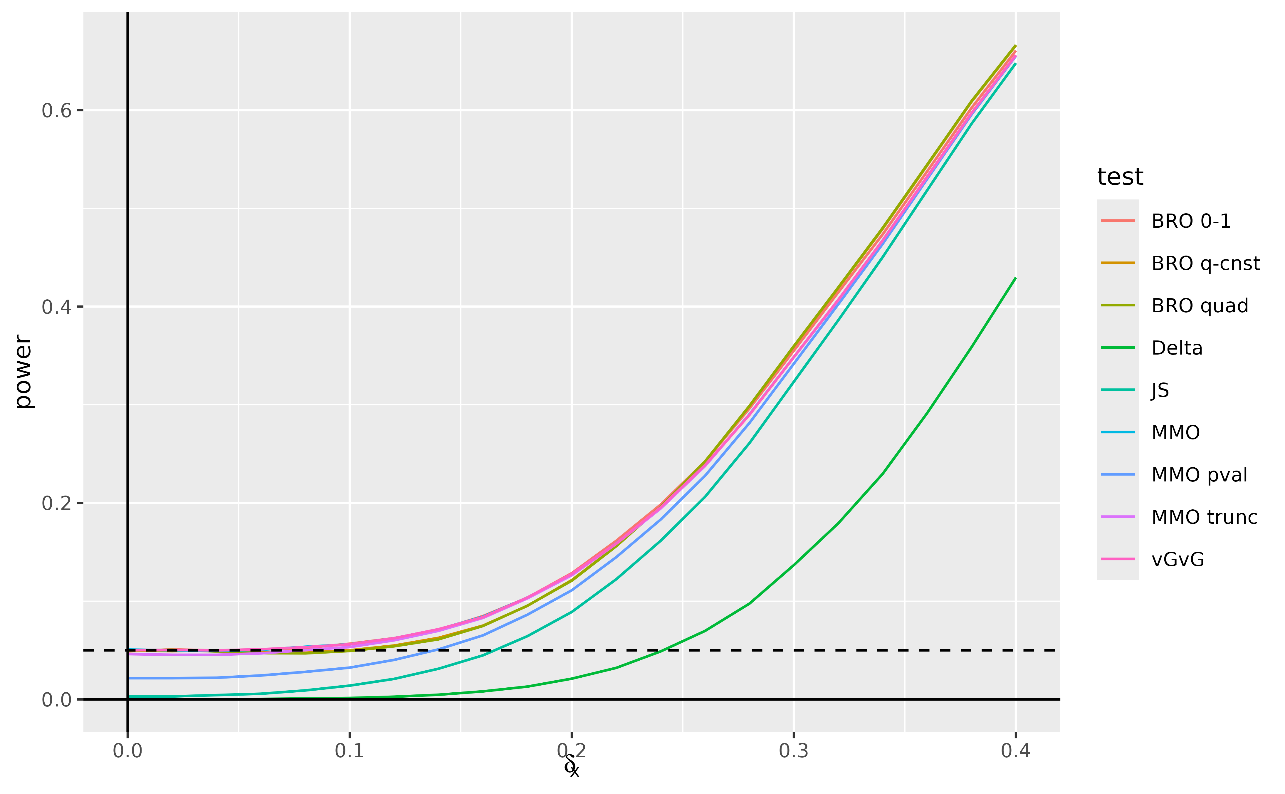

Apart from the minimax optimal $p$ -value-based test, all of the minimax optimal and Bayes risk optimal tests and the vGvG test have very close to nominal type 1 error at $(\delta_x,\delta_y)=(0,0)$ . All of these tests greatly outperform the delta method and joint significance tests in terms of power for smaller values of $\delta_x=\delta_y$ , with the minimax optimal $p$ -value-based test having power somewhere in between, but converging more quickly to the other tests.

The delta method test remains very conservative over the entire range of parameter values. All of the tests except for the delta method test begin to converge in power closer to 0.4. The minimax optimal (apart from the $p$ -value based test), Bayes risk optimal, and vGvG tests perform very similarly over the range of parameter values, with the quadratic loss versions of the Bayes risk optimal test trading off some power loss in the 0.1–0.2 range for a slight improvement in power in the 0.3–0.4 range, demonstrating the greater emphasis the quadratic loss places on larger alternatives. The truncated minimax optimal test begins slightly conservative relative to 0.05, but catches up with the most powerful tests fairly quickly.

Despite not being similar tests, the Bayes risk optimal and vGvG tests suffer very little in terms of power near the least favorable distribution at $(\delta_x,\delta_y)=(0,0)$ .

3 Scenario (b)

We now turn to scenario (b).

delta_x <- seq(0, .6, length.out = P + 1)
delta_y <- rep(.2, length(delta_x))

## ###################### ##
## running the simulation ##
## ###################### ##
pow_b <- run_simulation()

## ####################### ##
## colllecting the results ##
## ####################### ##
pow_scenario_b <- tibble(delta = rep(delta_x, 9),
                         power = unlist(pow_b),
                         test = c(rep("MMO", P + 1),
                                  rep("MMO trunc", P + 1),
                                  rep("BRO 0-1", P + 1),
                                  rep("BRO quad", P + 1),
                                  rep("BRO q-cnst", P + 1),
                                  rep("Delta", P + 1),
                                  rep("JS", P + 1),
                                  rep("MMO pval", P + 1),
                                  rep("vGvG", P + 1)))

fig_scenario_b <- ggplot(data = pow_scenario_b) + 
    geom_line(aes(
        x = delta, y = power, group = test,
        color = test,
        ),
        linewidth = 0.5) + 
    geom_vline(xintercept = 0) + 
    geom_hline(yintercept = 0) + 
    geom_hline(yintercept = alpha, linetype = "dashed") +
    xlab(expression(delta[x]))
(fig_scenario_b)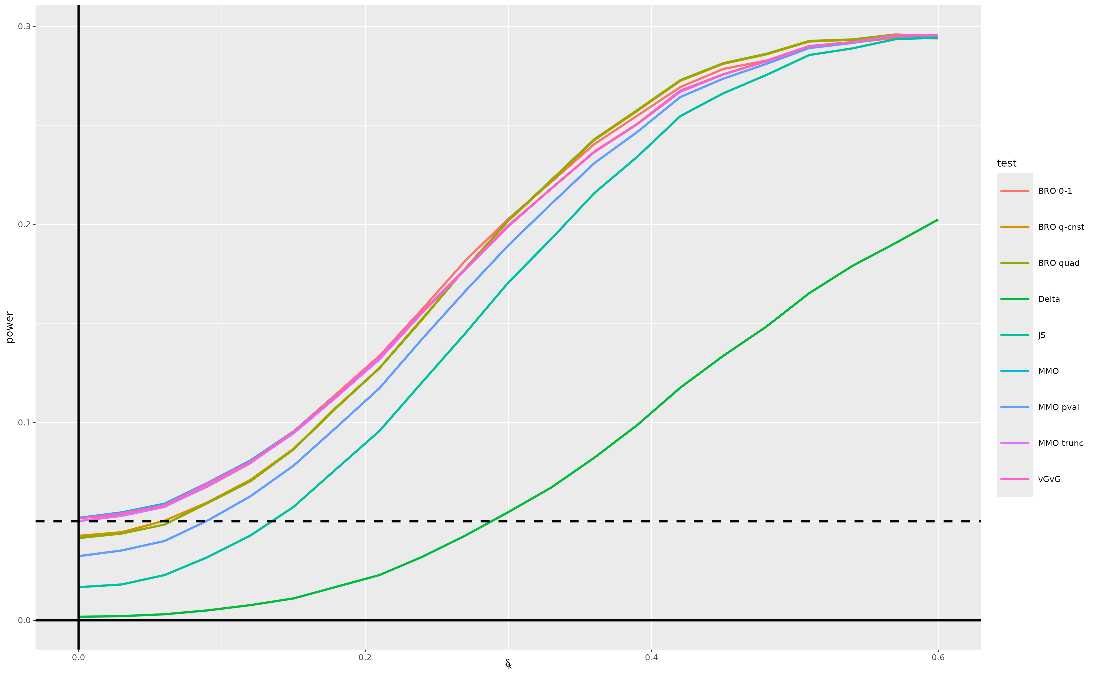

The trends are largely the same as in scenario (a). The main difference is that the quadratic loss versions of the Bayes risk optimal test are slightly conservative with respect to 0.05 under the null, albeit less conservative than the minimax optimal $p$ -value-based test.

Once again, these tests trade off some power loss for smaller values of $\delta_x$ (values less than about 0.25) for slightly improved power for larger values of $\delta_x$ (from about 0.35–0.55). Since $\delta_y$ is fixed at 0.2, power for all tests appears to plateau a little under 0.3.

4 Scenario (c)

We now turn to scenario (c).

delta_x <- seq(0, .8, length.out = P + 1)
delta_y <- rep(0, length(delta_x))

## ###################### ##
## running the simulation ##
## ###################### ##
pow_c <- run_simulation()

## ####################### ##
## colllecting the results ##
## ####################### ##
pow_scenario_c <- tibble(delta = rep(delta_x, 9),
                         power = unlist(pow_c),
                         test = c(rep("MMO", P + 1),
                                  rep("MMO trunc", P + 1),
                                  rep("BRO 0-1", P + 1),
                                  rep("BRO quad", P + 1),
                                  rep("BRO q-cnst", P + 1),
                                  rep("Delta", P + 1),
                                  rep("JS", P + 1),
                                  rep("MMO pval", P + 1),
                                  rep("vGvG", P + 1)))

fig_scenario_c <- ggplot(data = pow_scenario_c) + 
    geom_line(aes(
        x = delta, y = power, group = test,
        color = test,
        ),
        linewidth = 0.5) + 
    geom_vline(xintercept = 0) + 
    geom_hline(yintercept = 0) + 
    geom_hline(yintercept = alpha, linetype = "dashed") +
    xlab(expression(delta[x]))
(fig_scenario_c)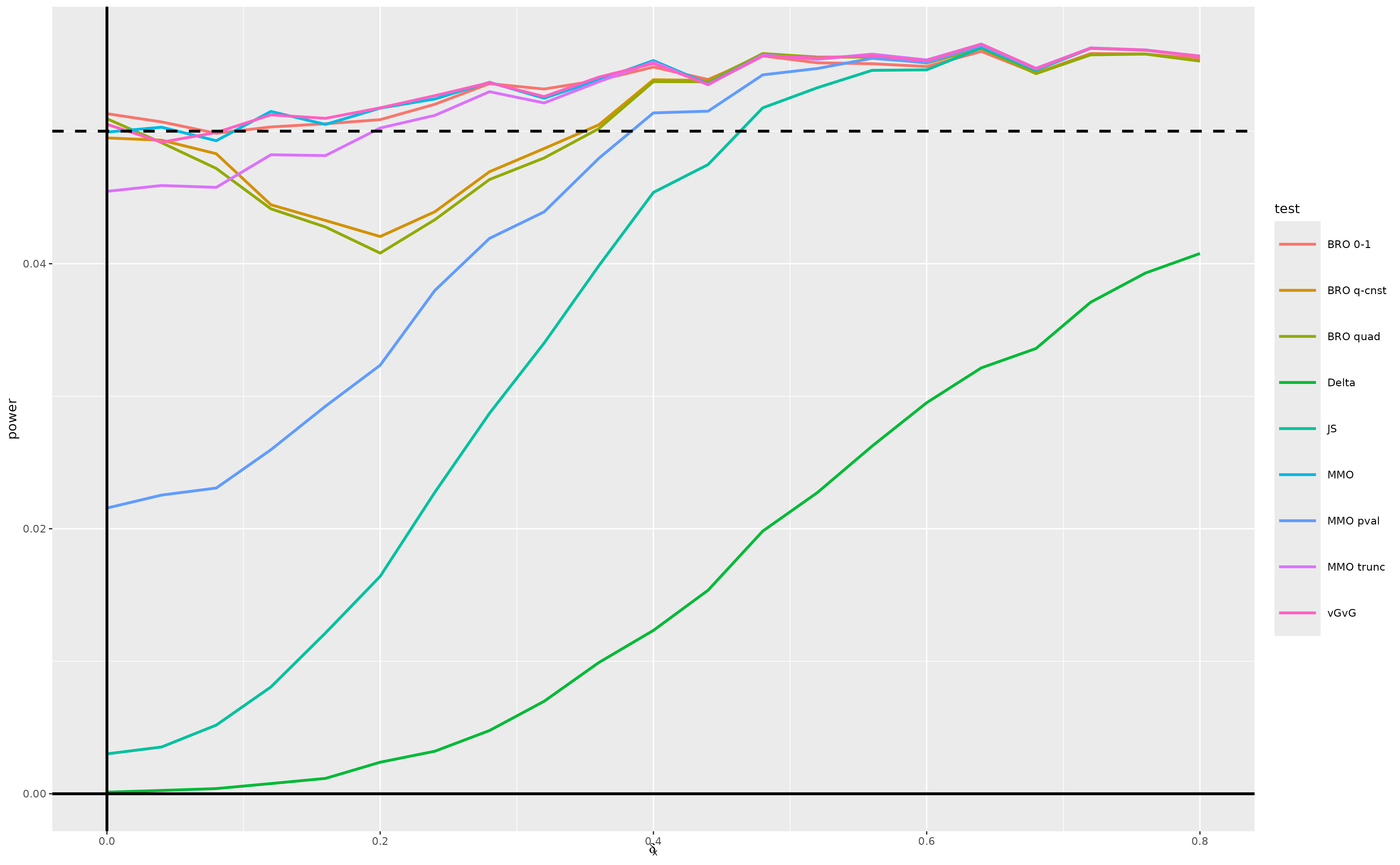

All tests approximately preserve type 1 error. Moreover, the performances of all tests except the delta method test converge by around $\delta_x=0.55$ .

However, the minimax optimal test exhibits some anti-conservative behavior due to the normal approximation being a bit too concentrated for a sample size of 50. This motivates conducting again the simulation study in scenario (c), substituting a $t$ -distribution for the standard normal approximation – see the next section.

5 Scenario (c) revisited

We revisit scenario (c), using a $t$ -distribution with $(n-1)$ degrees of freedom instead of the standard normal approximation in the minimax optimal tests. For this purpose, we simply redefine the object quantile_function.

delta_x <- seq(0, .8, length.out = P + 1)
delta_y <- rep(0, length(delta_x))

sample_size <- as.integer(n_obs - 1)
quantile_function <- \(t) qt(t, df = sample_size)

## ###################### ##
## running the simulation ##
## ###################### ##
pow_d <- run_simulation()

## ####################### ##
## colllecting the results ##
## ####################### ##
pow_scenario_d <- tibble(delta = rep(delta_x, 9),
                         power = unlist(pow_d),
                         test = c(rep("MMO", P + 1),
                                  rep("MMO trunc", P + 1),
                                  rep("BRO 0-1", P + 1),
                                  rep("BRO quad", P + 1),
                                  rep("BRO q-cnst", P + 1),
                                  rep("Delta", P + 1),
                                  rep("JS", P + 1),
                                  rep("MMO pval", P + 1),
                                  rep("vGvG", P + 1)))

fig_scenario_d <- ggplot(data = pow_scenario_d) + 
    geom_line(aes(
        x = delta, y = power, group = test,
        color = test,
        ),
        linewidth = 0.5) + 
    geom_vline(xintercept = 0) + 
    geom_hline(yintercept = 0) + 
    geom_hline(yintercept = alpha, linetype = "dashed") +
    xlab(expression(delta[x]))
(fig_scenario_d)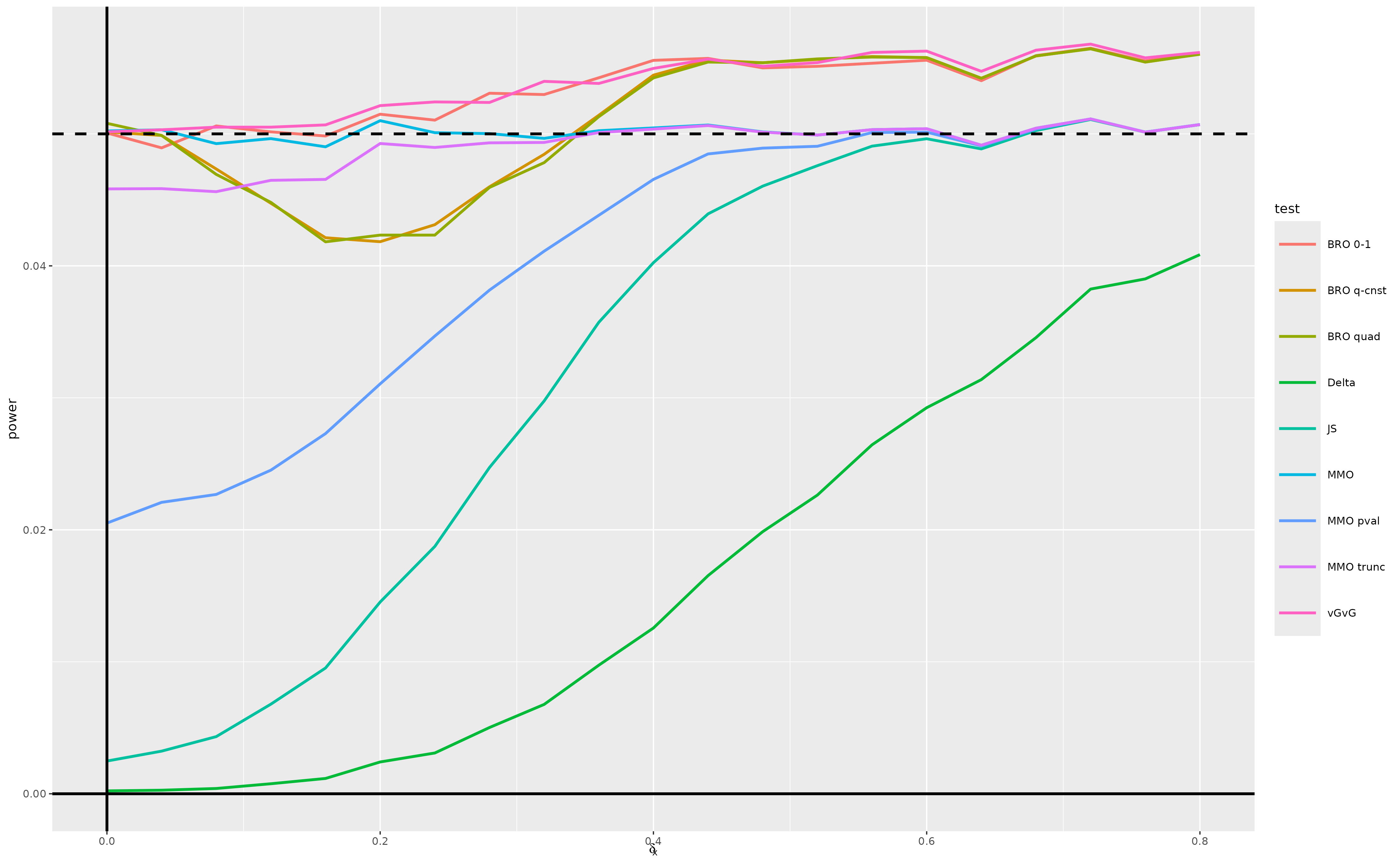

The use of the $t$ -distribution approximation has the expected effect. The type 1 error is now much closer to 0.05 across the entire range of the null hypothesis parameter space we consider. Again, the performances of all tests except the delta method converge by around $\delta_x=0.55$ .

References

Garderen, Kees Jan van, and Noud van Giersbergen. 2022. “A Nearly Similar Powerful Test for Mediation.” arXiv Preprint arXiv:2012.11342. https://arxiv.org/abs/2012.11342.

Miles, Caleb H., and Antoine Chambaz. 2024. “Optimal Tests of the Composite Null Hypothesis Arising in Mediation Analysis.” https://arxiv.org/abs/2107.07575.