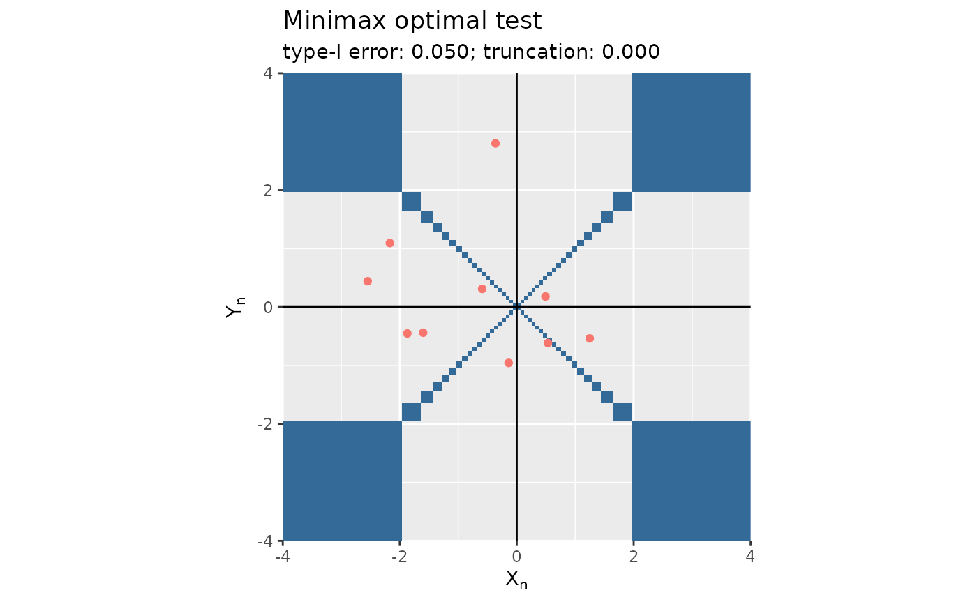
Plots the output of functions mediation_test_minimax and mediation_test_Bayes with the rejection region.
plot.mediation.test.RdPlots the output of functions mediation_test_minimax and mediation_test_Bayes with the rejection region.
Arguments
- x
An output of
functionsmediation_test_minimaxormediation_test_Bayes.- filename
Either
NULL(defaults) or a file name to create on disk.- return_fig
A
logical, to request that the 'ggplot2' object be returned (if 'TRUE') or not (if 'FALSE').- xlim, ylim
Two
vectorsofnumerics, the wished x-axis and y-axis ranges (both default to 'c(-4, 4)').- ...
Not used.
Value
Nothing unless 'return_fig' is set to 'TRUE', in which case the function returns the 'ggplot2' object.
Examples
n <- 10
x <- MASS::mvrnorm(n, mu = c(0, 0), Sigma = diag(c(1, 1)))
delta <- matrix(stats::runif(2 * n, min = -3, max = 3), ncol = 2)
epsilon <- stats::rbinom(n, 1, 1/2)
delta <- delta * cbind(epsilon, 1 - epsilon)
x <- x + delta
(mt <- mediation_test_minimax(x, alpha = 1/20))
#> Testing the composite null 'delta_x * delta_y = 0' against its alternative 'delta_x * delta_y != 0':
#> * method:
#> minimax
#> * test statictic:
#>            [,1]       [,2]
#> [1,] -2.1693445  3.2190488
#> [2,] -0.1391305 -1.0342846
#> [3,] -1.3763265  2.8520753
#> [4,]  2.8078932  1.4040790
#> [5,] -1.5349158 -0.5940126
#> [6,]  1.7506718  1.0603957
#> ...
#> * wished type-I error:
#> [1] 0.05
#> * user-supplied truncation parameter:
#> [1] 0
#> * size  of the sample used to derive the  test statistic ('Inf' to use a Gaussian approximation; otherwise, use a product of Student laws):
#> [1] Inf
#> * decision [1 rejection(s) overall]:
#> can reject the null for its alternative with confidence 0.050
#>  cannot reject the null for its alternative with confidence 0.050
#>  cannot reject the null for its alternative with confidence 0.050
#>  cannot reject the null for its alternative with confidence 0.050
#>  cannot reject the null for its alternative with confidence 0.050
#>  cannot reject the null for its alternative with confidence 0.050
#> ...
#> * (conservative) p-value:
#> [1] 0.03005654 0.88934702 0.16872056 0.16029533 0.55250367 0.28896464
#> ...
plot(mt)
